Optimizing sample sizes in A/B testing, Part II: Expected lift

10 Jan 2020

This is Part II of a three-part blog post on how to optimize your sample size in A/B testing. Make sure to read Part I if you haven’t already.

In this blog post (Part II), I describe what I think is an incredibly cool business-focused formula that quantifies how much you can benefit from increasing your sample size. It is, in short, an average of the value of all possible outcomes of the experiment, weighted by their probabilities. This post starts off kind of dry, but if you can make it through the first section, it gets a lot easier.

Outcome probabilities

Imagine you are comparing two versions of a website. You currently are on version A, but you would like to compare it to version B. Imagine you are measuring some random variable \(X\), which might represent something like clicks per user or page views per user. The goal of the experiment is to determine which version of the website has a higher mean value of \(X\).

This blog post aims to quantify the benefit of experimentation as an average of the value of all possible outcomes, weighted by their probabilities. To do that, we first need to describe the probabilities of all the different outcomes. An outcome consists of two parts: A true difference in means, \(\Delta\), defined as

\[\Delta = \mu_B - \mu_A\]

and an experimentally observed difference in means \(\delta\), defined as

\[\delta = \overline{X}_B - \overline{X}_A\]

Let’s start with \(\Delta\). While you don’t yet know which version of the website is better (that’s what the experiment is for!), you have a sense for how important the product change is. You can therefore create a normally distributed prior on \(\Delta\) with mean zero and variance \(\sigma_\Delta^2\).

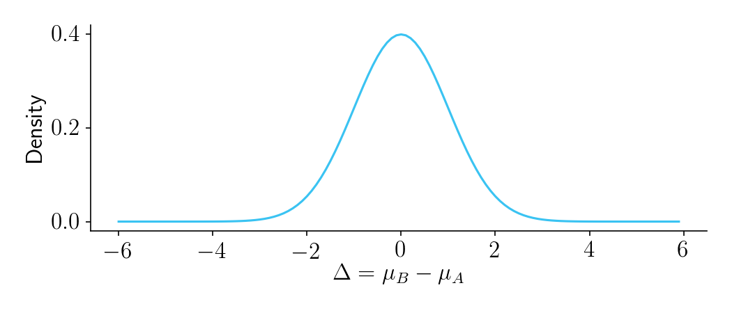
Figure 1.

Next, let’s consider \(\delta\), your experimentally observed difference in means. It will be a noisy estimate of \(\Delta\). Let’s assume you have previously measured the variance of \(X\) to be \(\sigma_X^2\). It is reasonable to assume that within each group in the experiment, and for any particular \(\Delta\), the variance of \(X\) will still be \(\sigma_X^2\). You should therefore believe that for any particular \(\Delta\), the observed difference in means \(\delta\) will be sampled from a normal distribution \(\mathcal{N}(\Delta, \sigma_c^2)\), where

\[\sigma_c^2 = \frac{2\sigma_X^2}{n}\]

and where \(n\) is the sample size in each of the two buckets. If that doesn’t make sense, check out this video.

Collectively, this all forms a bivariate normal distribution of outcomes, shown below.

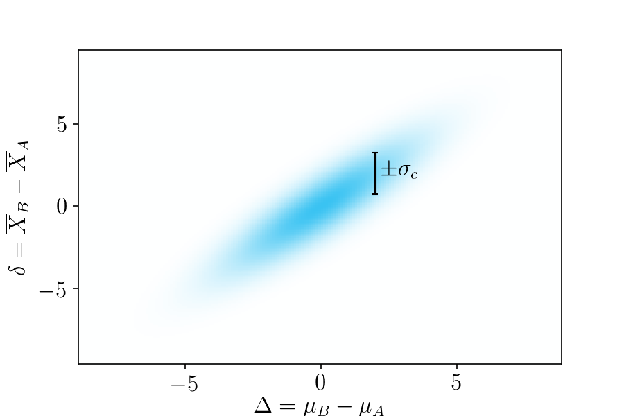
Figure 2. Probabilities of possible outcomes, based on your prior beliefs. The horizontal axis is the true difference in means, and the vertical axis is the observed difference in means.

To gain some more intuition about this, take a look at Figure 3. As sample size increases, \(\sigma^2_c\) decreases.

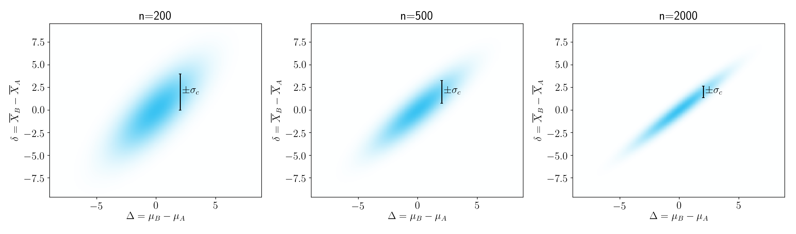
Figure 3.

Outcome lifts

Now that we know the probabilities of all the different outcomes, we next need to estimate how much per-user lift, \(l\), we will gain from each possible outcome, assuming we follow a policy of shipping whichever bucket (A or B) looked better in the experiment.

In cases where \(\delta > 0\) and \(\Delta > 0\), you would ship B and your post-experiment per-user lift will be positively valued at \(l = \Delta\).
In cases where \(\delta > 0\) and \(\Delta < 0\), you would ship B, but unfortunately your post-experiment per-user lift will be negatively valued at \(l = \Delta\), since \(\Delta\) is negative.
In cases where \(\delta < 0\), you would keep A in production, and your post-experiment lift would be zero.

A heatmap of the per-user lifts (\(l\)) for each outcome is shown in the plot below. Good outcomes, where shipping B was the right decision, are shown in blue. Bad outcomes, where shipping B was the wrong decision, are shown in red. There are two main ways to get a neutral outcomes, shown in white. Either you keep A (bottom segment), in which case there is zero lift, or you ship B where B is only negligibly different than A (vertical white stripe).

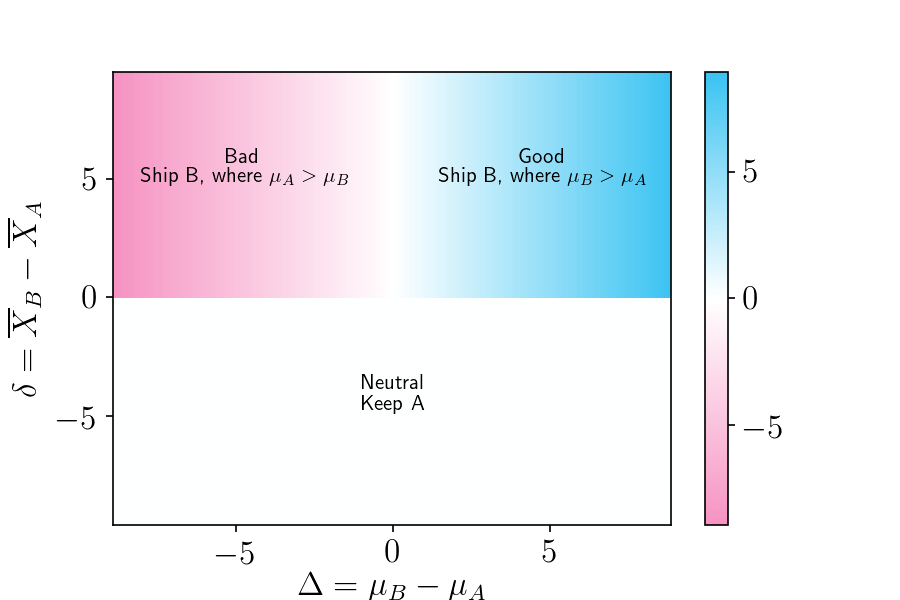
Figure 4. Heatmap of possible outcomes, where the color scale represents the lift. The horizontal axis is the true difference in means, and the vertical axis the observed difference in means

Probability-weighted Outcome Lifts

At this point, we know the probability of each outcome, and we know the post-experiment per-user lift of each outcome. To determine how much lift we can expect, on average, by shipping the winning bucket of an experiment, we need to compute a probability-weighted average of the outcome lifts. Let’s start by looking at this visually and then later we’ll get into the math.

As shown in Figure 5, if we multiply the bivariate normal distribution (left) by the lift map (center), we can obtain the probability-weighted lift of each outcome (right).

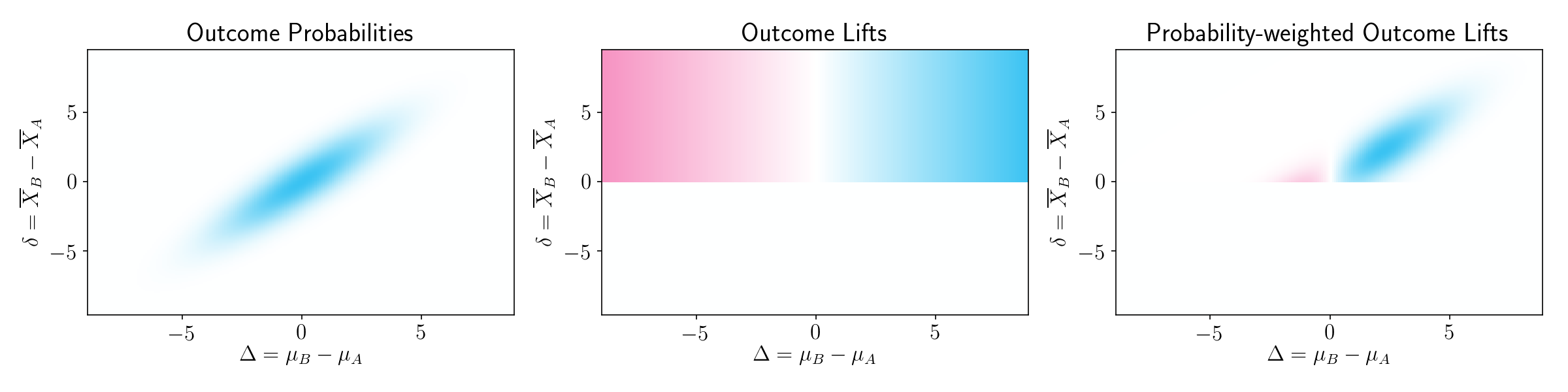
Figure 5.

The good outcomes contribute more than the bad outcomes, simply because a good outcome is more likely than a bad outcome. To put it differently, experimentation will on average give you useful information.

To gain some more intuition on this, it is helpful to see this plot for different sample sizes. As sample size increases, the probability-weighted contribution of bad outcomes gets smaller and smaller.

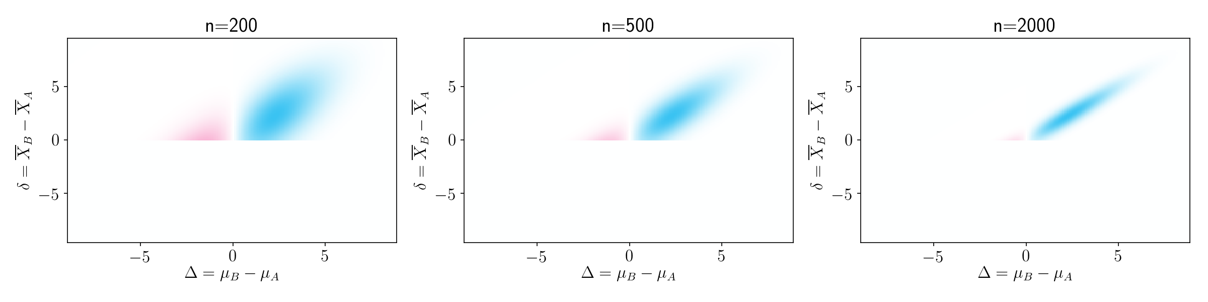
Figure 6.

Computing the expected post-experiment per-user lift

We’re almost there! To determine the expected post-experiment lift from shipping the winning bucket, we need to compute a probability-weighted average of all the post-experiment lifts. In other words, we need to sum up all the probability-weighted post-experiment lifts on the right panel of Figure 5. The formula for doing this is shown below. A derivation can be found in the Appendix.

\[\hat{L} = \frac{\sigma_\Delta^2}{\sqrt{2\pi(\sigma_\Delta^2 + \frac{2\sigma_X^2}{n})}}\]

There’s three things to notice about this formula.

As \(n\) increases, \(\hat{L}\) increases. This makes sense. The larger the sample size, the more likely it is that you’ll ship the winning bucket.
As the within-group variance \(\sigma_X^2\) increases, \(\hat{L}\) decreases. That’s because a high within-group variance makes experiments less informative – they’re more likely to give you the wrong answer.
As the variance prior on \(\Delta\) increases, \(\hat{L}\) increases. This also make sense. The more impactful (positive or negative) you think the product change might be, the more value you will get from experimentation.

You can try this out using the get_lift_via_closed_form formula in the Notebook.

Demonstration via simulation

In the previous section, we derived a formula for \(\hat{L}\). Should you trust a formula you found on a random internet blog? Yes! Let’s put the formula to the test, by comparing its predictions to actual simulations.

First, let’s consider the case where the outcome is a continuous variable, such as the number of clicks. Let’s set \(\sigma_D^2 = 2\) and \(\sigma_X^2 = 100\). We then measure \(\hat{L}\) for a range of sample sizes, using both the closed-form solution and simulations. To see how we determine \(\hat{L}\) for simulations, refer to the box below.

Procedure for finding \(\hat{L}\) with simulations

Loop through thousands of simulated experiments. On each each experiment doing the following:

Sample a true group difference \(\Delta\) from \(\mathcal{N}(0, \sigma_D^2)\)
Sample an \(X\) for each of the \(n\) users in each bucket A and B, using Normal distributions \(\mathcal{N}(\frac{\Delta}{2}, \sigma_X^2)\) and \(\mathcal{N}(-\frac{\Delta}{2}, \sigma_X^2)\), respectively.
Compute \(\delta = \overline{X}_B - \overline{X}_A\).
If \(\delta <= 0\), stick with A and accrue zero lift.
If \(\delta > 0\), ship B and accrue the per-user lift of \(\Delta\), which will probably, but not necessarily, be positive.

We run these experiments thousands of times, each time computing the per-user lift. Finally, we average all the per-user lifts together to get \(\hat{L}\). See the get_lift_via_simulations_continuous function in the notebook for an implementation.

As seen in Figure 7, below, the results of the simulation closely match the closed-form solution.

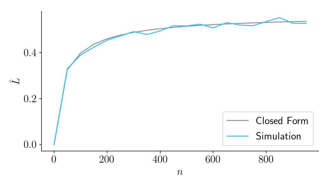
Figure 7.

Second, let’s consider the case where the variable is binary, as in conversion rates. For reasonably large values of \(n\), we can safely assume that the error variance is normally distributed with variance \(\sigma_X^2 = p(1-p)\), where \(p\) is the baseline conversion rate. For this example, let’s set the baseline conversion rate \(p = 0.1\), and let’s set \(\sigma_\Delta^2 = 0.01^2\). The results of the simulation closely match the closed-form solution.

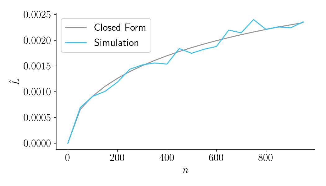
Figure 8.

Thinking about costs, and a preview of Part III

In this blog post, we saw how increasing the sample size improves the expected post-experiment per-user lift, \(\hat{L}\). But to determine the optimal sample size, we need to think about costs.

The cost in dollars of an experiment can be described as \(f + vn\), where \(f\) is a fixed cost and \(v\) is the variable cost per participant. If you already know these costs, and if you already know the revenue increase \(u\) from each unit increase in lift, you can calculate the net revenue \(R\) as

\[R = u\hat{L} - f - vn\]

and then find the sample size \(n\) that maximizes \(R\).

Unfortunately, these costs aren’t always readily available. The good news is that there is a really nice way to calculate the most important cost: the forfeited benefit that comes from prolonging your experiment. To read about that, and about how to optimize your sample size, please continue to Part III.

Appendix

To determine \(\hat{L}\), we start with the probability-weighted lifts on the right panel of Figure 5. This is a bivariate normal distribution over \(\Delta\) and \(\delta\), multiplied by \(\Delta\).

\[f(\Delta, \delta) = \frac{\Delta}{2 \pi \sigma_\Delta \sigma_\delta \sqrt{1-\rho^2}} e^{-\frac{ \frac{\Delta^2}{\sigma_\Delta^2} - \frac{2 \rho \Delta \delta}{\sigma_\Delta \sigma_\delta} + \frac{\delta^2}{\sigma_\delta^2} }{2(1-\rho^2)} }\]

where the correlation coefficient \(\rho\), is defined as:

\[\rho = \sqrt{1 - \frac{\sigma_c^2}{\sigma_\Delta^2 + \sigma_c^2}}\]

and \(\sigma_\delta^2\) is the variance on \(\delta\). By the variance addition rules, \(\sigma_\delta^2\) is defined as

\[\sigma_\delta^2 = \sigma_\Delta^2 + \sigma_c^2\]

We next need to sum up the probability-weighted values in \(f(\Delta, \delta)\). To obtain a closed form solution, we can use integration.

\[\hat{L} = \int_{0}^{\infty} \int_{-\infty}^{\infty} {\frac{\Delta}{2 \pi \sigma_\Delta \sigma_\delta \sqrt{1-\rho^2}} e^{-\frac{ \frac{\Delta^2}{\sigma_\Delta^2} - \frac{2 \rho \Delta \delta}{\sigma_\Delta \sigma_\delta} + \frac{\delta^2}{\sigma_\delta^2} }{2(1-\rho^2)} } \,d\Delta\,d\delta }\]

The integration limits on \(\delta\) start at zero because the lift will always be zero if \(\delta < 0\) (i.e if the status quo bucket A wins the experiment).

Thanks to my 15-day free trial of Mathematica, I determined that this integral comes out to the surprisingly simple

\[\hat{L} = \rho \frac{\sigma_\Delta}{\sqrt{2\pi}}\]

The command I used was:

Integrate[(t / (2*\[Pi]*s1*s2*Sqrt[1 - p^2]))*Exp[-((t^2/s1^2 - \
(2*p*t*d)/(s1*s2) + d^2/s2^2)/(2*(1 - p^2)))], {d, 0, \[Infinity]}, \
{t, -\[Infinity], \[Infinity]}, Assumptions -> p > 0 && p < 1 && s1 > \
0 && s2 > 0]

If we then substitute in previously defined formulas for \(\rho\) and \(\sigma_c^2\), we can produce a formula that accepts more readily-available inputs.