
Variance after scaling and summing: One of the most useful facts from statistics
18 May 2019What do \(R^2\), laboratory error analysis, ensemble learning, meta-analysis, and financial portfolio risk all have in common? The answer is that they all depend on a fundamental principle of statistics that is not as widely known as it should be. Once this principle is understood, a lot of stuff starts to make more sense.
Here’s a sneak peek at what the principle is.
\[\sigma_{p}^{2} = \sum\limits_{i} \sum\limits_{j} w_i w_j \sigma_i \sigma_j \rho_{ij}\]Don’t worry if the formula doesn’t yet make sense! We’ll work our way up to it slowly, taking pit stops along the way at simpler formulas that are useful on their own. As we work through these principles, we’ll encounter lots of neat applications and explainers.
This post consists of three parts:
- Part 1: Sums of uncorrelated random variables: Applications to social science and laboratory error analysis
- Part 2: Weighted sums of uncorrelated random variables: Applications to machine learning and scientific meta-analysis
- Part 3: Correlated variables and Modern Portfolio Theory
Part 1: Sums of uncorrelated random variables: Applications to social science and laboratory error analysis
Let’s start with some simplifying conditions and assume that we are dealing with uncorrelated random variables. If you take two of them and add them together, the variance of their sum will equal the sum of their variances. This is amazing!
To demonstrate this, I’ve written some Python code that generates three arrays, each of length 1 million. The first two arrays contain samples from two normal distributions with variances 9 and 16, respectively. The third array is the sum of the first two arrays. As shown in the simulation, its variance is 25, which is equal to the sum of the variances of the first two arrays (9 + 16).
from numpy.random import randn
import numpy as np
n = 1000000
x1 = np.sqrt(9) * randn(n) # 1M samples from normal distribution with variance=9
print(x1.var()) # 9
x2 = np.sqrt(16) * randn(n) # 1M samples from normal distribution with variance=16
print(x2.var()) # 16
xp = x1 + x2
print(xp.var()) # 25
This fact was first discovered in 1853 and is known as Bienaymé’s Formula. While the code example above shows the sum of two random variables, the formula can be extended to multiple random variables as follows:
If \(X_p\) is a sum of uncorrelated random variables \(X_1 .. X_n\), then the variance of \(X_p\) will be
\[\sigma_{p}^{2} = \sum{\sigma^2_i}\]where each \(X_i\) has variance \(\sigma_i^2\).
What does the \(p\) stand for in \(X_p\)? It stands for portfolio, which is just one of the many applications we’ll see later in this post.
Why this is useful
Bienaymé’s result is surprising and unintuitive. But since it’s such a simple formula, it is worth committing to memory, especially because it sheds light on so many other principles. Let’s look at two of them.
Understanding \(R^2\) and “variance explained”
Psychologists often talk about “within-group variance”, “between-group variance”, and “variance explained”. What do these terms mean?
Imagine a hypothetical study that measured the extraversion of 10 boys and 10 girls, where extraversion is measured on a 10-point scale (Figure 1. Orange bars). The boys have a mean extraversion of 4.4 and the girls have a mean extraversion 5.0. In addition, the overall variance of the data is 2.5. We can decompose this variance into two parts:
- Between-group variance: Create a 20-element array where every boy is assigned to the mean boy extraversion of 4.4, and every girl is assigned to the mean girl extraversion of 5.0. The variance of this array is 0.9. (Figure 1. Blue bars).
- Within-group variance: Create a 20-element array of the amount each child’s extraversion deviates from the mean value for their sex. Some of these values will be negative and some will be positive. The variance of this array is 1.6. (Figure 1. Pink bars).
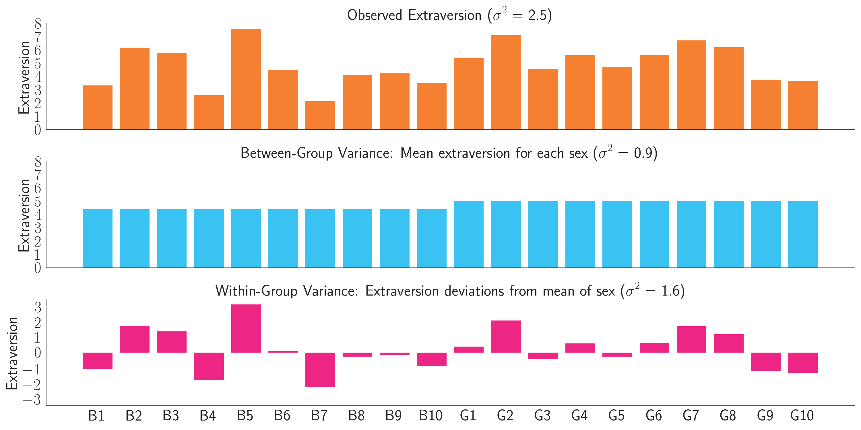
Figure 1: Decomposition of extraversion scores (orange) into between-group variance (blue) and within-group variance (pink).
If you add these arrays together, the resulting array will represent the observed data (Figure 1. Orange bars). The variance of the observed array is 2.5, which is exactly what is predicted by Bienaymé’s Formula. It is the sum of the variances of the two component arrays (0.9 + 1.6). Psychologists might say that sex “explains” 0.9/2.5 = 36% of the extraversion variance. Equivalently, a model of extraversion that uses sex as the only predictor would have an \(R^2\) of 0.36.
Error propagation in laboratories
If you ever took a physics lab or chemistry lab back in college, you may remember having to perform error analysis, in which you calculated how errors would propagate through one noisy measurement after another.
Physics textbooks often say that standard deviations add in “quadrature”, which just means that if you are trying to estimate some quantity that is the sum of two other measurements, and if each measurement has some error with standard deviation \(\sigma_1\) and \(\sigma_2\) respectively, the final standard deviation would be \(\sigma_{p} = \sqrt{\sigma^2_1 + \sigma^2_2}\). I think it’s probably easier to just use variances, as in the Bienaymé Formula, with \(\sigma^2_{p} = \sigma^2_1 + \sigma^2_2\).
For example, imagine you are trying to estimate the height of two boxes stacked on top of each other (Figure 2). One box has a height of 1 meter with variance \(\sigma^2_1\) = 0.01, and the other has a height of 2 meters with variance \(\sigma^2_2\) = 0.01. Let’s further assume, perhaps optimistically, that these errors are independent. That is, if the measurement of the first box is too high, it’s not any more likely that the measurement of the second box will also be too high. If we can make these assumptions, then the total height of the two boxes will be 3 meters with variance \(\sigma^2_p\) = 0.02.
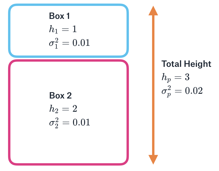
Figure 2: Two boxes stacked on top of each other. The height of each box is measured with some variance (uncertainty). The total height is the sum of the individual heights, and the total variance (uncertainty) is the sum of the individual variances.
There is a key difference between the extraversion example and the stacked boxes example. In the extraversion example, we added two arrays that each had an observed sample variance. In the stacked boxes example, we added two scalar measurements, where the variance of these measurements refers to our measurement uncertainty. Since both cases have a meaningful concept of ‘variance’, the Bienaymé Formula applies to both.
Part 2: Weighted sums of uncorrelated random variables: Applications to machine learning and scientific meta-analysis
Let’s now move on to the case of weighted sums of uncorrelated random variables. But before we get there, we first need to understand what happens to variance when a random variable is scaled.
If \(X_p\) is defined as \(X\) scaled by a factor of \(w\), then the variance \(X_p\) will be
\[\sigma_{p}^{2} = w^2 \sigma^2\]where \(\sigma^2\) is the variance of \(X\).
This means that if a random variable is scaled, the scale factor on the variance will change quadratically. Let’s see this in code.
from numpy.random import randn
import numpy as np
n = 1000000
baseline_var = 10
w = 0.7
x1 = np.sqrt(baseline_var) * randn(n) # Array of 1M samples from normal distribution with variance=10
print(x1.var()) # 10
xp = w * x1 # Scale this by w=0.7
print(w**2 * baseline_var) # 4.9 (predicted variance)
print(xp.var()) # 4.9 (empirical variance)
To gain some intuition for this rule, it’s helpful to think about outliers. We know that outliers have a huge effect on variance. That’s because the formula used to compute variance, \(\sum{\frac{(x_i - \bar{x})^2}{n-1}}\), squares all the deviations, and so we get really big variances when we square large deviations. With that as background, let’s think about what happens if we scale our data by 2. The outliers will spread out twice as far, which means they will have even more than twice as much impact on the variance. Similarly, if we multiply our data by 0.5, we will squash the most “damaging” part of the outliers, and so we will reduce our variance by more than a factor of two.
While the above principle is pretty simple, things start to get interesting when you combine it with the Bienaymé Formula in Part I:
If \(X_p\) is a weighted sum of uncorrelated random variables \(X_1 ... X_n\), then the variance of \(X_p\) will be
\[\sigma_{p}^{2} = \sum{w^2_i \sigma^2_i}\]where each \(w_i\) is a weight on \(X_i\), and each \(X_i\) has its own variance \(\sigma_i^2\).
The above formula shows what happens when you scale and then sum random variables. The final variance is the weighted sum of the original variances, where the weights are squares of the original weights. Let’s see how this can be applied to machine learning.
An ensemble model with equal weights
Imagine that you have built two separate models to predict car prices. While the models are unbiased, they have variance in their errors. That is, sometimes a model prediction will be too high, and sometimes a model prediction will be too low. Model 1 has a mean squared error (MSE) of $1,000 and Model 2 has an MSE of $2,000.
A valuable insight from machine learning is that you can often create a better model by simply averaging the predictions of other models. Let’s demonstrate this with simulations below.
from numpy.random import randn
import numpy as np
n = 1000000
actual = 20000 + 5000 * randn(n)
errors1 = np.sqrt(1000) * randn(n)
print(errors1.var()) # 1000
errors2 = np.sqrt(2000) * randn(n)
print(errors2.var()) # 2000

# Note that this section could be replaced with
# errors_ensemble = 0.5 * errors1 + 0.5 * errors2
preds1 = actual + errors1
preds2 = actual + errors2
preds_ensemble = 0.5 * preds1 + 0.5 * preds2
errors_ensemble = preds_ensemble - actual

print(errors_ensemble.var()) # 750. Lower than variance of component models!
As shown in the code above, even though a good model (Model 1) was averaged with an inferior model (Model 2), the resulting Ensemble model’s MSE of $750 is better than either of the models individually.
The benefits of ensembling follow directly from the weighted sum formula we saw above, \(\sigma_{p}^{2} = \sum{w^2_i \sigma^2_i}\). To understand why, it’s helpful to think of models not as generating predictions, but rather as generating errors. Since averaging the predictions of a model corresponds to averaging the errors of the model, we can treat each model’s array of errors as samples of a random variable whose variance can be plugged in to the formula. Assuming the models are unbiased (i.e. the errors average to about zero), the formula tells us the expected MSE of the ensemble predictions. In the example above, the MSE would be
\[\sigma_{p}^{2} = 0.5^2 \times 1000 + 0.5^2 \times 2000 = 750\]which is exactly what we observed in the simulations.
(For a totally different intuition of why ensembling works, see this blog post that I co-wrote for my company, Opendoor.)
An ensemble model with Inverse Variance Weighting
In the example above, we obtained good results by using an equally-weighted average of the two models. But can we do better?
Yes we can! Since Model 1 was better than Model 2, we should probably put more weight on Model 1. But of course we shouldn’t put all our weight on it, because then we would throw away the demonstrably useful information from Model 2. The optimal weight must be somewhere in between 50% and 100%.
An effective way to find the optimal weight is to build another model on top of these models. However, if you can make certain assumptions (unbiased and uncorrelated errors), there’s an even simpler approach that is great for back-of-the envelope calculations and great for understanding the principles behind ensembling.
To find the optimal weights (assuming unbiased and uncorrelated errors), we need to minimize the variance of the ensemble errors \(\sigma_{p}^{2} = \sum{w^2_i \sigma^2_i}\) with the constraint that \(\sum{w_i} = 1\).
It turns out that the variance-minimizing weight for a model should be proportional to the inverse of its variance.
\[w_k = \frac{\frac{1}{\sigma^2_k}}{\sum{\frac{1}{\sigma^2_i}}}\]When we apply this method, we obtain optimal weights of \(w_1\) = 0.67 and \(w_2\) = 0.33. These weights give us an ensemble error variance of
\[\sigma_{p}^{2} = 0.67^2 \times 1000 + 0.33^2 \times 2000 = 666\]which is significantly better than the $750 variance we were getting with equal weighting.
This method is called Inverse Variance Weighting, and allows you to assign the right amount of weight to each model, depending on its error.
Inverse Variance Weighting is not just useful as a way to understand Machine Learning ensembles. It is also one of the core principles in scientific meta-analysis, which is popular in medicine and the social sciences. When multiple scientific studies attempt to estimate some quantity, and each study has a different sample size (and hence variance of their estimate), a meta-analysis should weight the high sample size studies more. Inverse Variance Weighting is used to determine those weights.
Part 3: Correlated variables and Modern Portfolio Theory
Let’s imagine we now have three unbiased models with the following MSEs:
- Model 1: MSE = 1000
- Model 2: MSE = 1000
- Model 3: MSE = 2000
By Inverse Variance Weighting, we should assign more weight to the first two models, with \(w_1=0.4, w_2=0.4, w_3=0.2\).
But what happens if Model 1 and Model 2 have correlated errors? For example, whenever Model 2’s predictions are too high, Model 3’s predictions tend to also be too high. In that case, maybe we don’t want to give so much weight to Models 1 and 2, since they provide somewhat redundant information. Instead we might want to diversify our ensemble by increasing the weight on Model 3, since it provides new independent information.
To determine how much weight to put on each model, we first need to determine how much total variance there will be if the errors are correlated. To do this, we need to borrow a formula from the financial literature, which extends the formulas we’ve worked with before. This is the formula we’ve been waiting for.
If \(X_p\) is a weighted sum of (correlated or uncorrelated) random variables \(X_1 ... X_n\), then the variance of \(X_p\) will be
\[\sigma_{p}^{2} = \sum\limits_{i} \sum\limits_{j} w_i w_j \sigma_i \sigma_j \rho_{ij}\]where each \(w_i\) and \(w_j\) are weights assigned to \(X_i\) and \(X_j\), where each \(X_i\) and \(X_j\) have standard deviations \(\sigma_i\) and \(\sigma_j\), and where the correlation between \(X_i\) and \(X_j\) is \(\rho_{ij}\).
There’s a lot to unpack here, so let’s take this step by step.
- \(\sigma_i \sigma_j \rho_{ij}\) is a scalar quantity representing the covariance between \(X_i\) and \(X_j\).
- If none of the variables are correlated with each other, then all the cases where \(i \neq j\) will go to zero, and the formula reduces to \(\sigma_{p}^{2} = \sum{w^2_i \sigma^2_i}\), which we have seen before.
- The more that two variables \(X_i\) and \(X_j\) are correlated, the more the total variance \(\sigma_{p}^{2}\) increases.
- If two variables \(X_i\) and \(X_j\) are anti-correlated, then the total variance decreases, since \(\sigma_i \sigma_j \rho_{ij}\) is negative.
- This formula can be rewritten in more compact notation as \(\sigma_{p}^{2} = \vec{w}^T\Sigma \vec{w}\), where \(\vec{w}\) is the weight vector, and \(\Sigma\) is the covariance matrix (not a summation sign!)
If you skimmed the bullet points above, go back and re-read them! They are super important.
To find the set of weights that minimize variance in the errors, you must minimize the above formula, with the constraint that \(\sum{w_i} = 1\). One way to do this is to use a numerical optimization method. In practice, however, it is more common to just find weights by building another model on top of the base models
Regardless of how the weights are found, it will usually be the case that if Models 1 and 2 are correlated, the optimal weights will reduce redundancy and put lower weight on these models than simple Inverse Variance Weighting would suggest.
Applications to financial portfolios
The formula above was discovered by economist Harry Markowitz in his Modern Portfolio Theory, which describes how an investor can optimally trade off between expected returns and expected risk, often measured as variance. In particular, the theory shows how to maximize expected return given a fixed variance, or minimize variance given a fixed expected return. We’ll focus on the latter.
Imagine you have three stocks to put in your portfolio. You plan to sell them at time \(T\), at which point you expect that Stock 1 will have gone up by 5%, with some uncertainty. You can describe your uncertainty as variance, and in the case of Stock 1, let’s say \(\sigma_1^2\) = 1. This stock, as well Stocks 2 and 3, are summarized in the table below:
| Stock ID | Expected Return | Expected Risk (\(\sigma^2\)) |
|---|---|---|
| 1 | 5.0 | 1.0 |
| 2 | 5.0 | 1.0 |
| 3 | 5.0 | 2.0 |
This financial example should remind you of ensembling in machine learning. In the case of ensembling, we wanted to minimize variance of the weighted sum of error arrays. In the case of financial portfolios, we want to minimize the variance of the weighted sum of scalar financial returns.
As before, if there are no correlations between the expected returns (i.e. if Stock 1 exceeding 5% return does not imply that Stock 2 or Stock 3 will exceed 5% return), then the total variance in the portfolio will be \(\sigma_{p}^{2} = \sum{w^2_i \sigma^2_i}\) and we can use Inverse Variance Weighting to obtain weights \(w_1=0.4, w_2=0.4, w_3=0.2\).
However, sometimes stocks have correlated expected returns. For example, if two of the stocks are in oil companies, then one stock exceeding 5% implies the other is also likely to exceed 5%. When this happens, the total variance becomes
\[\sigma_{p}^{2} = \sum\limits_{i} \sum\limits_{j} w_i w_j \sigma_i \sigma_j \rho_{ij}\]as we saw before in the ensemble example. Since this includes an additional positive term for \(w_1 w_2 \sigma_1 \sigma_2 \rho_{1,2}\), the expected variance is higher than in the uncorrelated case, assuming the correlations are positive. To reduce this variance, we should put less weight on Stocks 1 and 2 than we would otherwise.
While the example above focused on minimizing the variance of a financial portfolio, you might also be interested in having a portfolio with high return. Modern Portfolio Theory describes how a portfolio can reach any abitrary point on the efficient frontier of variance and return, but that’s outside the scope of this blog post. And as you might expect, financial markets can be more complicated than Modern Portfolio Theory suggests, but that’s also outside scope.
Summary
That was a long post, but I hope that the principles described have been informative. It may be helpful to summarize them in backwards order, starting with the most general principle.
If \(X_p\) is a weighted sum of (correlated or uncorrelated) random variables \(X_1 ... X_n\), then the variance of \(X_p\) will be
\[\sigma_{p}^{2} = \sum\limits_{i} \sum\limits_{j} w_i w_j \sigma_i \sigma_j \rho_{ij}\]where each \(w_i\) and \(w_j\) are weights assigned to \(X_i\) and \(X_j\), where each \(X_i\) and \(X_j\) have standard deviations \(\sigma_i\) and \(\sigma_j\), and where the correlation between \(X_i\) and \(X_j\) is \(\rho_{ij}\). The term \(\sigma_i \sigma_j \rho_{ij}\) is a scalar quantity representing the covariance between \(X_i\) and \(X_j\).
If none of the variables are correlated, then all the cases where \(i \neq j\) go to zero, and the formula reduces to
\[\sigma_{p}^{2} = \sum{w^2_i \sigma^2_i}\]And finally, if we are computing a simple sum of random variables where all the weights are 1, then the formula reduces to
\[\sigma_{p}^{2} = \sum{\sigma^2_i}\]