
Optimizing sample sizes in A/B testing, Part III: Aggregate time-discounted expected lift
10 Jan 2020This is Part III of a three part blog post on how to optimize your sample size in A/B testing. Make sure to read Part I and Part II if you haven’t already.
In Part II, we learned how before the experiment starts we can estimate \(\hat{L}\), the expected post-experiment lift, a probability weighted average of outcomes.
In Part III, we’ll discuss how to estimate what is perhaps the most important per-unit cost of experimentation: the forfeited benefits that are lost by delayed shipment. This leads to something I think is incredibly cool: A formula for the aggregate time-discounted expected post-experiment lift as a function of sample size. We call this quantity \(\hat{L}_a\). The formula for \(\hat{L}_a\) allows you to pick optimal sample sizes specific to your business circumstances. We’ll cover two examples in Python, one where you are testing a continuous variable, and one where you are testing a binary variable (as in conversion rate experiments).
As usual, the focus will be on choosing a sample size at the beginning of the experiment and committing to it, not on dynamically updating the sample size as the experiment proceeds.
A quick modification from Part II
In Part II, we saw that if you ship whichever version (A or B) does best in the experiment, your business will on average experience a post-experiment per-user lift of
\[\hat{L} = \frac{\sigma_\Delta^2}{\sqrt{2\pi(\sigma_\Delta^2 + \frac{2\sigma_X^2}{n})}}\]where \(\sigma_\Delta^2\) is the variance on your normally distributed zero-mean prior for \(\mu_B - \mu_A\), \(\sigma_X^2\) is the within-group variance, and \(n\) is the per-bucket sample size.
Because Part III is primarily concerned with the duration of the experiment, we’re going to modify the formula to be time-dependent. As a simplifying assumption we’re going to make sessions, rather then users, the unit of analysis. We’ll also assume that you have a constant number of sessions per day. This changes the definition of \(\hat{L}\) to a post-experiment per-session lift, and the formula becomes
\[\hat{L} = \frac{\sigma_\Delta^2}{\sqrt{2\pi(\sigma_\Delta^2 + \frac{2\sigma_X^2}{m\tau})}}\]where \(m\) is the sessions per day for each bucket, and \(\tau\) is duration of the experiment in days.
Time Discounting
The formula above shows that larger sample sizes result in higher \(\hat{L}\), since larger samples make it more likely you will ship the better version. But as with all things in life, there are costs to increasing your sample size. In particular, the larger your sample size, the longer you have to wait to ship the winning bucket. This is bad because lift today is much more valuable than the same lift a year from now.
How much more valuable is lift today versus lift a year from now? A common way to quantify this is with exponential discounting, such that weights (or “discount factors”) on future lift follow the form:
\[w = e^{-rt}\]where \(r\) is a discount rate. For startup teams, the annual discount rate might be quite large, like 0.5 or even 1.0, which would correspond to a daily discount rate \(r\) of 0.5/365 or 1.0/365, respectively. Figure 1 shows an example of a discount rate of 1.0/365
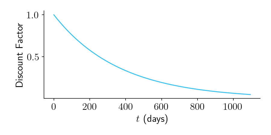
Figure 1.
Aggregate time-discounted expected lift: Visual Intuition
Take a look at Figure 2, below. It shows an experiment that is planned to run for \(\tau = 60\) days. The top panel shows \(\hat{L}\), which we have now defined as the expected per-session lift. While the experiment is running, \(\hat{L} = 0\), since our prior is that \(\Delta\) is sampled from a normal distribution with mean zero. But once the experiment finishes and we launch the winning bucket, we should begin to reap our expected per-session lift.
The middle panel shows our discount function.
The bottom panel shows our time-discounted lift, defined as the product of the lift in the top panel and the time discount in the middle panel. (We can also multiply it by \(M\), the number of post-experiment sessions per day, which for simplicity we set to 1 here.) The aggregate time-discounted expected lift, \(\hat{L}_a\), is the area under the curve.
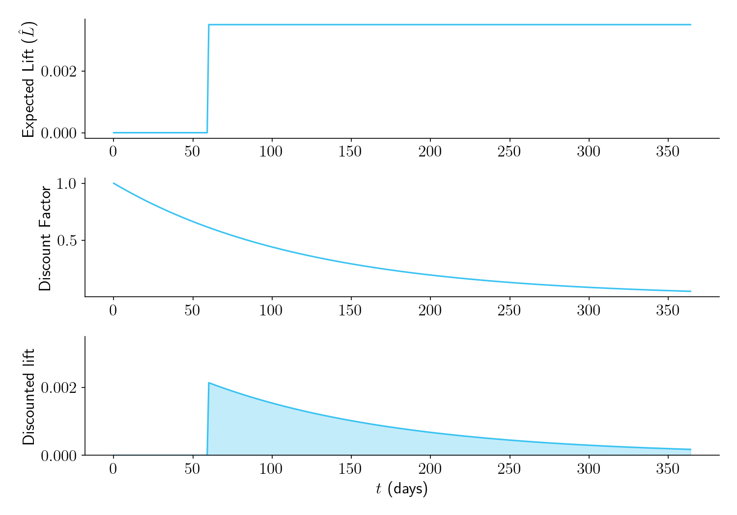
Figure 2.
Now let’s see what happens with different experiment durations. Figure 3 shows that the longer you plan to run your experiment, the higher \(\hat{L}\) will be (top panel). But due to time discounting, (middle panel), the area under the time-discounted lift curve (bottom panel) is low for overly large sample sizes. There is an optimal duration of the experiment (in this case, \(\tau = 24\) days), that maximizes \(\hat{L}_a\), the area under the curve.
Figure 3.
Aggregate time-discounted expected lift: Formula
The aggregate time-discounted expected lift \(\hat{L}_a\), i.e. the area under the curve in the bottom panel of Figure 3, is:
\[\hat{L}_a = \frac{\sigma_\Delta^2 M e^{-r\tau}}{r \sqrt{2\pi(\sigma_\Delta^2 + \frac{2\sigma_X^2}{m\tau})}}\]where \(\tau\) is the duration of the experiment and \(M\) is the number of post-experiment sessions per day. See the Appendix for a derivation.
There’s two things to note about this formula.
- Increasing the number of bucketed sessions per day, \(m\), always increases \(\hat{L}_a\).
- Increasing the duration of the experiment, \(\tau\), may or may not help. Its impact is controlled by competing forces in the numerator and denominator. In the numerator, higher \(\tau\) decreases \(\hat{L}_a\) by delaying shipment. In the denominator, higher \(\tau\) increases \(\hat{L}_a\) by making it more likely you will ship the superior version.
Optimizing sample size
At long last, we can answer the question, “How long should we run this experiment?”. A nice way to do it is to plot \(\hat{L}_a\) as a function of \(\tau\). Below we see what this looks like for one set of parameters. Here the optimal duration is 38 days.
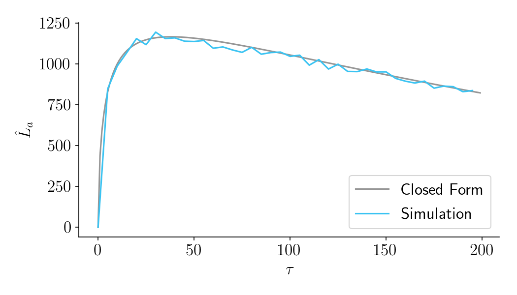
Figure 4.
Note also that a set of simulated experiment and post-experiment periods (in blue) confirm the predictions of the closed form solution (in gray). See the notebook for details.
Examples in Python
Example 1: Continuous variable metric
Let’s say you want to run an experiment comparing two different versions of a website, and your main metric is revenue per session. You know in advance that the within-group variance of this metric is \(\sigma_X^2 = 100\). You don’t know which version is better but you have a prior that the true difference in means is normally distributed with variance \(\sigma_\Delta^2 = 1\). You have 200 sessions per day and plan to bucket 100 sessions into Version A and 100 sessions into Version B, running the experiment for \(\tau=20\) days. Your discount rate is fairly aggressive at 1.0 annually, or \(r = 1/365\) per day. Using the function in the notebook, you can find \(\hat{L}_a\) with this command:
get_agg_lift_via_closed_form(var_D=1, var_X=100, m=100, tau=25, r=1/365, M=200)
# returns 26298
You can also use the find_optimal_tau function to determine the optimal duration, which in this case is \(\tau=18\).
Example 2: Conversion rates
Let’s say your main metric is conversion rate. You think that on average conversion rates will be about 10%, and that the difference in conversion rates between buckets will be normally distributed with variance 1%. Using the normal approximation of the binomial distribution, you can use p*(1-p) for var_X.
p = 0.1
get_agg_lift_via_closed_form(var_D=0.01**2, var_X=p*(1-p), m=100, tau=25, r=1/365, M=200)
# returns 207
You can also use the find_optimal_tau function to determine the optimal duration, which in this case is \(\tau=49\).
FAQ
Q: Has there been any similar work on this?
A: As I was writing this, I came across a fantastic in-press paper by Elea Feit and Ron Berman. The paper is exceptionally clear and I would recommend reading it. Like this blog post, Feit and Berman argue that it doesn’t make any sense to pick sample sizes based on statistical significance and power thresholds. Instead they recommend profit-maximizing sample sizes. They independently come to the same formula for \(\hat{L}\) as I do (see right addend in their Equation 9, making sure to substitute my \(\frac{\sigma_\Delta^2}{2}\) for their \(\sigma^2)\). Where they differ is that they assume there is a fixed pool of \(N\) users that can only experience the product once. In their setup, you can allocate \(n_1\) users to Bucket A and \(n_2\) users to Bucket B. Once you have identified the winning bucket, you ship that version to the remaining \(N-n_1-n_2\) users. Your expected profit is determined by the total expected lift from those users. My experience in industry differs from this setup. In my experience there is no constraint that you can only show the product once to a fixed set of users. Instead, there is often an indefinitely increasing pool of new users, and once you ship the winning bucket you can ship it to everyone, including users who already participated in the experiment. To me, the main constraint in industry is therefore time discounting, rather than a finite pool of users.
Q: In addition to the lift from shipping a winning bucket, doesn’t experimentation also help inform us about the types of products that might work in the future? And if so, doesn’t this mean we should run experiments longer than recommended by your formula for \(\hat{L}_a\)?
A: Yes, experimentation can teach lessons that are generalizable beyond the particular product being tested. This is an advantage of high powered experimentation not included in my framework.
Q: What about novelty effects?
A: Yup, that’s a real concern not covered by my framework. You probably want to know a somewhat long term impact of your product, which means you should probably run the experiment for longer than recommended by my framework.
Q: If some users can show up in multiple sessions, doesn’t bucketing by session violate independence assumptions?
A: Yeah, so this is tricky. For many companies, there is a distribution of user activity, where some users come for many sessions per week and other users come for only one session at most. Modeling this would make the framework significantly more complicated, so I tried to simplify things by making sessions the unit of analysis.
Q: Is there anything else on your blog vaguely related to this topic?
A: I’m glad you asked!
- Four pitfalls of hill climbing discusses some product-focused issues in A/B testing
- Hyperbolic discounting — The irrational behavior that might be rational after all is about time discounting, although not in the context of experimentation.
Appendix
The aggregate time-discounted expected lift \(\hat{L}_a\) is
\[\hat{L}_a = \int_{\tau}^{\infty} \hat{L} M e^{-rt} \,dt\]where \(\hat{L}\) is the expected per-session lift, \(M\) is the number of post-experiment sessions per day, \(r\) is the discount rate, and \(\tau\) is the duration of the experiment. Solving the integral gives:
\[\hat{L}_a = \frac{\hat{L} M e^{-r\tau}}{r}\]Plugging in our previously solved value of \(\hat{L}\) gives
\[\hat{L}_a = \frac{\sigma_\Delta^2 M e^{-r\tau}}{r \sqrt{2\pi(\sigma_\Delta^2 + \frac{2\sigma_X^2}{m\tau})}}\]