Optimizing sample sizes in A/B testing, Part I: General summary

10 Jan 2020

---

If you’re a data scientist, you’ve surely encountered the question, “How big should this A/B test be?”

The standard answer is to do a power analysis, typically aiming for 80% power at \(\alpha\)=5%. But if you think about it, this advice is pretty weird. Why is 80% power the best choice for your business? And doesn’t a 5% significance cutoff seem pretty arbitrary?

In most business decisions, you want to choose a policy that maximizes your benefits minus your costs. In experimentation, the benefit comes from learning information to drive future decisions, and the cost comes from the experiment itself. The optimal sample size will therefore depend on the unique circumstances of your business, not on arbitrary statistical significance thresholds.

In this three-part blog post, I’ll present a new way of determining optimal sample sizes that completely abandons the notion of statistical significance.

• Part I: General Overview. Starts with a mostly non-technical overview and ends with a section called “Three lessons for practitioners”.
• Part II: Expected lift. A more technical section that quantifies the benefits of experimentation as a function of sample size.
• Part III: Aggregate time-discounted lift. A more technical section that quantifies the costs of experimentation as a function of sample size. It then combines costs and benefits into a closed-form expression that can be optimized. Ends with an FAQ.

Throughout Parts I-III, the focus will be on choosing a sample size at the beginning of the experiment and committing to it, not on dynamically updating the sample size as the experiment proceeds.

With that out of the way, let’s get started!

Benefits of large samples

The bigger your sample size, the more likely it is that you’ll ship the right bucket. Since there is a gain to shipping the right bucket and a loss to shipping the wrong bucket, the average benefit of the experiment is a probability-weighted average of these outcomes. We call this the expected post-experiment lift, \(\hat{L}\), which increases with sample size. We’ll cover this in more detail in Part II.

Costs of large samples

For most businesses, increasing your sample size requires you to run your experiment longer. This brings us to the main per-unit cost of experimentation: the forfeited benefits that could come from shipping the winning bucket earlier. In a fast moving startup, there’s often good reason to accrue your wins as soon as possible. The advantage of shipping earlier can be quantified with a discount rate, which describes how much you value the near future over the distant future. If you have a high discount rate, it’s critical to ship as soon as possible. If you have a low discount rate, you can afford to wait longer. This is described in more detail in Part III.

Combining costs and benefits into an optimization function

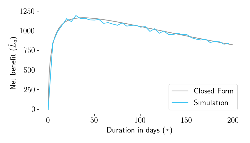
You should run your experiment long enough that you’ll likely ship the winning bucket, but not so long that you waste time not having shipped your product. The optimal duration depends on the unique circumstances of your business. The overall benefit of running an experiment, as a function of duration and other parameters, is defined as the aggregate time-discounted expected post-experiment lift, or \(\hat{L}_a\).

Figure 1 shows \(\hat{L}_a\) as a function of experiment duration in days (\(\tau\)) for one particular set of business parameters. The gray curve shows the result of a closed form solution presented in Part III. The blue curve shows the results of simulated experiments. As you can see, the optimal duration for this experiment should be about 38 days. Simulations match the closed-form predictions.

Three lessons for practitioners

I played around with the formula for \(\hat{L}_a\) and came across three lessons that should be of interest to practitioners.

1. You should run “underpowered” experiments if you have a very high discount rate

Take a look at Figure 2, which shows some recommendations for a fairly typical two-bucket conversion rate experiment with 1000 sessions per bucket per day. On the left panel we plot the optimal duration as a function of the annual discount rate. If you have a high discount rate, you care a lot more about the near future than the distant future. It is therefore critical that you ship any potentially winning version as soon as possible. In this scenario, the optimal duration is low (left panel). Power, the probability you will find a statistically significant result, is also low (right panel). For many of these cases, the optimal duration would traditionally be considered “underpowered”.

2. You should run “underpowered” experiments if you have a small user base

Now let’s plot these curves as a function of \(m\), our daily sessions per bucket. If you only have a small number of daily sessions to work with, you’ll need to run the experiment for longer (left panel). So far, that’s not surprising. But here’s where it gets interesting: Even though optimal duration increases as \(m\) decreases, it doesn’t increase fast enough to maintain constant power (right panel). In fact, for low \(m\) scenarios where you don’t have a lot of users, the optimal duration results in power that can drop below 50%, well into what would traditionally be considered “underpowered” territory. In these situations, waiting to get a large number of sessions causes too much time-discounting loss.

3. That said, it’s far better to run your experiment too long than too short

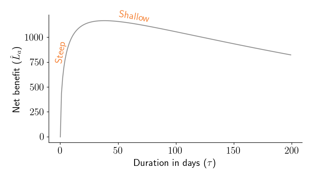
Let’s take another look at \(\hat{L}_a\) as a function of duration. As shown in Figure 4 below, the left shoulder is steeper than the right shoulder. This means that it’s really bad if your experiment is shorter than optimal, but it’s kind of ok if your experiment is longer than optimal.

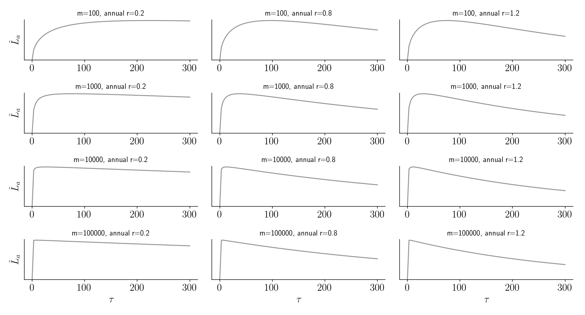
Is this true in general? Yes. Below we plot \(\hat{L}_a\) as a function of duration for various combinations of \(m\) and the discount rate, \(r\). For all of these parameter combinations, it’s better to run a bit longer than optimal than a bit shorter than optimal. The only exception is if you have an insanely high discount rate (not shown).

Upcoming posts and Python notebook

You probably have a lot of questions about where this framework comes from and how it is justified. Part II and Part III dive more deeply into the math and visual intuition behind it. They also contain some example uses of the get_lift_via_closed_form and get_agg_lift_via_closed_form functions available in the accompanying Python Notebook.