
The respiratory infection study to end all respiratory infection studies
11 Feb 2024[Notebook]
The most basic question one might have about respiratory infections like Covid is when are you infectious? Some researchers believe that people with low viral RNA counts like \(10^3\) cp/mL are meaningfully infectious\(^1\). Others believe that almost all spread occurs during the brief peak of viral count, at around \(10^9\) cp/mL. The answer will determine whether you typically stop being infectious after 8-9 days or something more like 1-2 days.
With over 700,000 papers published papers on Covid, you’d think we’d have a solid answer to such a basic and practically useful question. But the reality is we don’t. Some epidemiological papers have attempted to measure this. But since they can’t measure precisely when people were infected or even by whom, their estimates of infectiousness thresholds are biased downwards by an unknown amount.
The second most basic question someone might ask is how well does ventilation / filtration / UVC work? While there is broad agreement these might work a little bit, we do not have the type of precise quantitative estimate that is needed for rational decision making or investment. Will an air filter in a school room reduce infection by 2% or by 30%? Nobody knows! All we have are unconvincing non-experiments, and some experiments that test only part of the infection pathway, leaving us with much uncertainty.
To really nail an answer to these questions, we don’t need another hundred thousand unconvincing studies. We just need one study. It will be a single, career-defining study of historical importance that will live forever in textbooks and convince experts and laypeople alike. It will be a large experiment where infected participants (“donors”) get in a room with uninfected participants (“recipients”), and we measure how much transmission happens under experimentally manipulated conditions.
Concerned about ethics? Just use the common cold! If you model things right, you can generalize much of the findings to other viruses.
I’ve simulated this type of experiment pretty extensively (see code). This blog post proposes how to optimally design and analyze it.
How to design the experiment
Suppose you want to compare transmission rates under high ventilation versus low ventilation conditions. Modeling shows that donor viral count will dominate the effect of other variables, which makes it hard to detect ventilation effects without very large sample sizes. It’s therefore critical that the experiment controls this variation. Each donor should have a chance to infect participants in each condition. To further reduce variance, any variable you don’t want to measure (e.g. distance, duration, talking vs silence) should be held constant in all interactions. A schematic design is below.
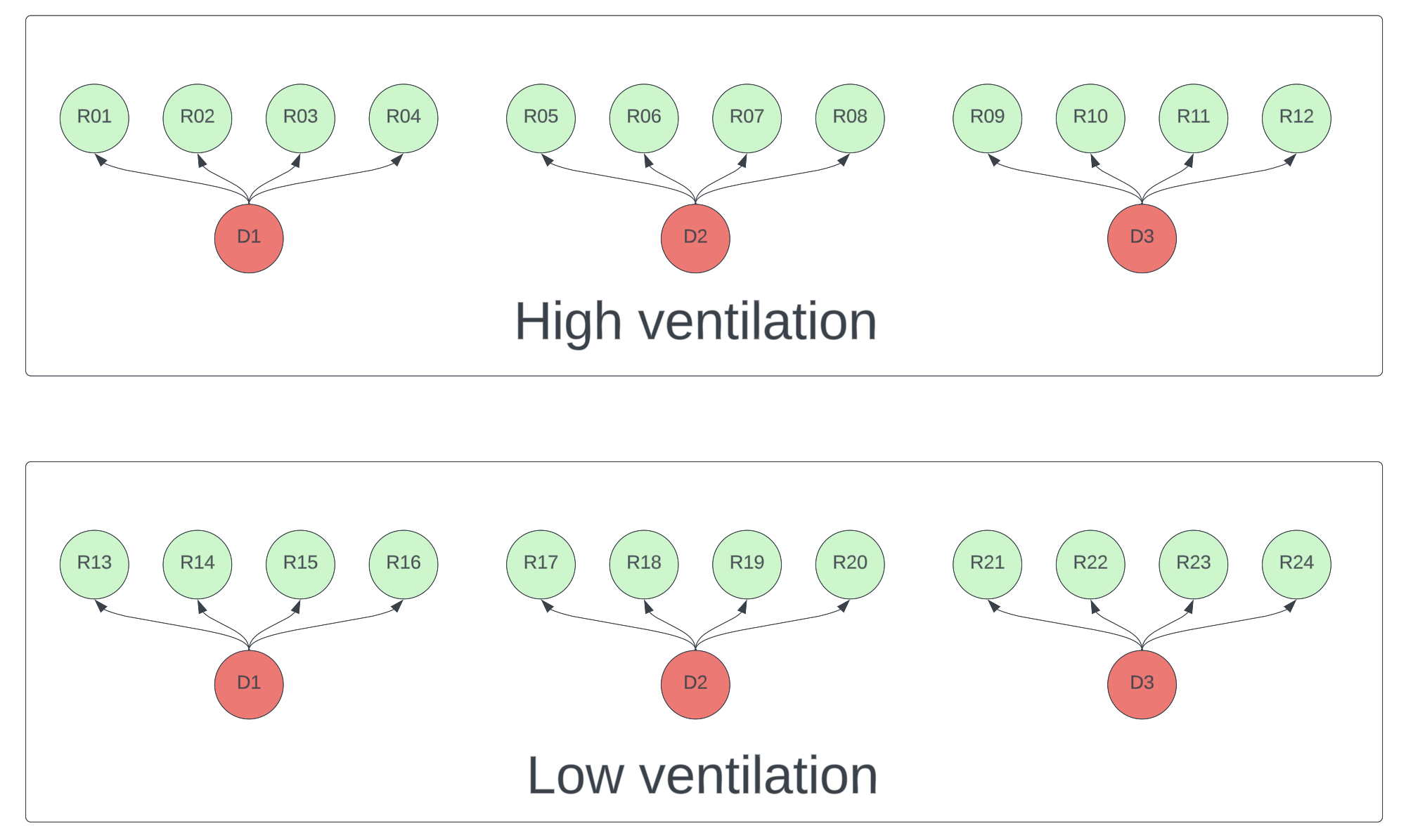
Figure 1. Schematic of a high ventilation vs low ventilation experiment. Each donor (red) must participate in both conditions. Each recipient (green) should only be exposed to one <donor, condition> pair.
How to model the results
The simplest and least useful way to analyze the results is to measure the infection rates in each condition. If you want to really reap the benefits of the experiment and enable yourself to quantitatively generalize to other interventions and even other viruses, you need to computationally model the data in the same way that transmission happens.
Under steady state conditions the amount of live virus inhaled per unit time is a linear function of the product of donor viral count, emission constants, filtration constants, and ventilation constants. This value is then scaled to a hazard rate of infection, via a scaling constant that depends on how easily each inhaled virus can cause an infection. As with any survival model, the probability of infection is an exponential function of this hazard rate.
For those who want to see the math, the probability of transmission between donor \(i\) and a recipient is
\[p_{i} = 1 - e^{-{\lambda}_{i}t}\]where the hazard rate \(\lambda_{i}\) is the product of donor viral count \(V_i\), and air quality and transmissibility constants captured in \(\beta\).
\[\lambda_{i} = \beta V_{i}\]In the figure below, I generated some simulated data and fit it with the model above. You can see how ventilation doesn’t matter for very low viral counts (when no one gets infected) or very high viral counts (where everyone gets infected), but it can help for intermediate viral counts.
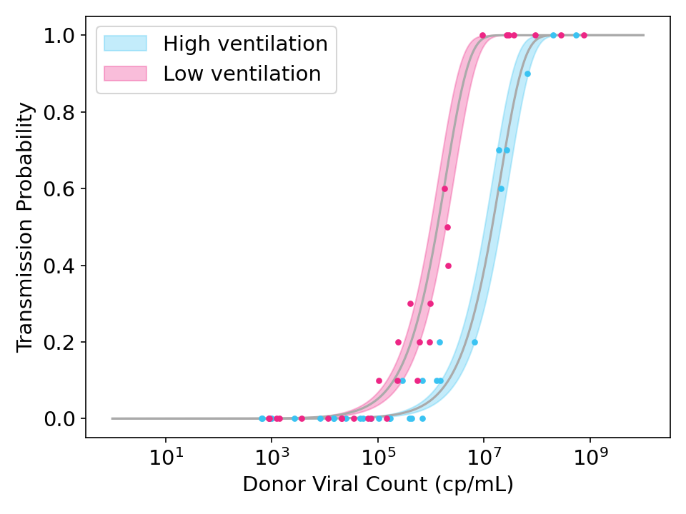
Figure 2: Simulated data and model fits showing the effect of strong ventilation designed to reduce viral concentration in the air by a factor of 10. Each point represents the transmission rate for donor exposed to 10 recipients. Shaded region is the 95% credible interval.
While the model above should work well if every recipient is equally susceptible, it may fail if there is variance in recipient susceptibilities. When this happens, the curve is flattened because highly susceptible recipients will get infected by low viral count donors and highly immune recipients will avoid infection even from high viral count donors.
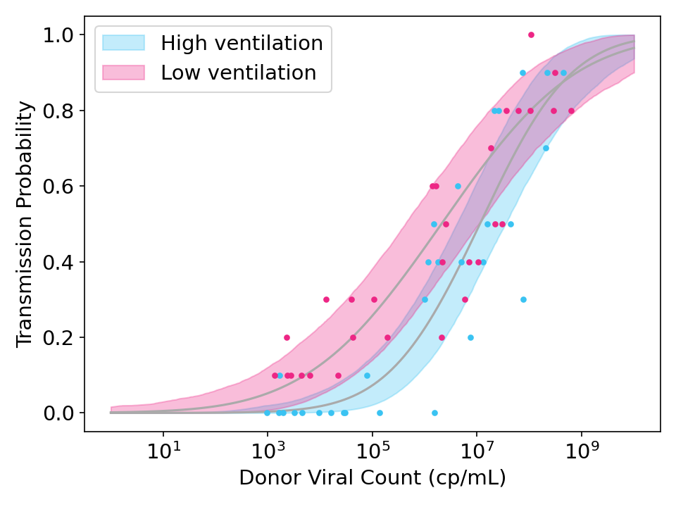
Figure 3: Simulated data showing the effect of strong ventilation designed to reduce viral concentration in the air by a factor of 10. Unlike Figure 2, the simulated data and model fits both allow for variation in the susceptibility of recipients.
To model this, I introduced a susceptibility variance term \(S_j\) to simulate the unknown variance in susceptibilities across participants, and fit it with hierarchical Bayesian methods (see code).
How many participants are needed?
If you don’t measure viral count or use each donor in each condition, you will need hundreds of donors and thousands of participants, which is infeasible, even for a 4x reduction in inhaled virus. But if each donor participates in all conditions and if you measure viral count, you can achieve 80% power with about 40 donors and 5 recipients per <donor, condition>. Getting donors is much more important than getting recipients, as there are diminishing returns for adding more participants after about 7-8 recipients per <donor, condition>.
The plots below show statistical power under various scenarios.
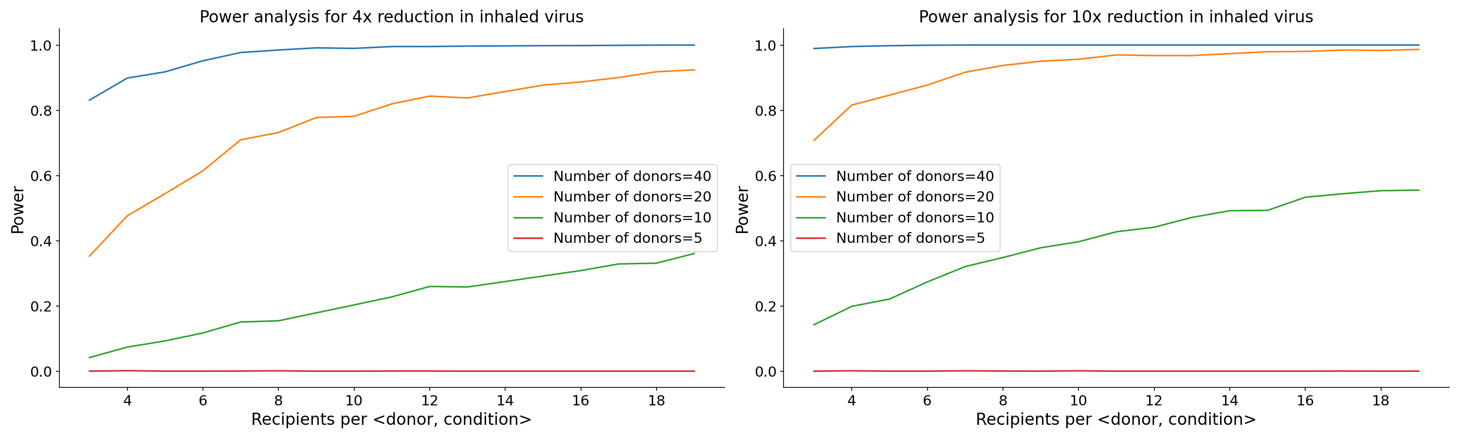
Figure 4. Power as a function of donor count and recipients per donor for an experiment that reduces viral concentration by a factor of 4 (left) and one that reduces viral concentration by a factor of 10 (right).
Generalizing to other interventions and other viruses
An experiment with 40 donors and 400 recipients is pretty expensive. But in addition to the primary benefits of telling us (1) when people are meaningfully infectious and (2) how well the tested intervention works, the experiment results can also be generalized to other interventions and even to other viruses!
The graph below shows the transmission probability / viral load curve for different values of \(\beta\), which is the product of several multiplicative terms (ventilation constants, filtration constants, constants, emission constants, baseline susceptibility). For every 10x you reduce viral concentration in the air (e.g. by increasing ventilation), the curve shifts right by one log.
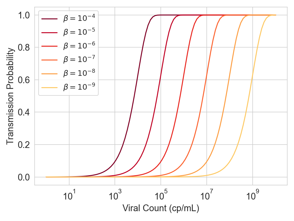
Figure 5. Infection probability as a function of viral count for various values of \(\beta\), which is a product of several multiplicative terms (ventilation constants, filtration constants, constants, emission constants, baseline susceptibility).
This means that you can generalize to other interventions.
- If ventilation can shift the curve by K logs, then increasing the ventilation to have an additional 10x reduction in viral concentration should shift the curve by K+1 logs.
- If a separate intervention like UVC provides the protection of ventilation plus an additional 10x reduction in viral concentration, then it should also shift the curve by K+1 logs.
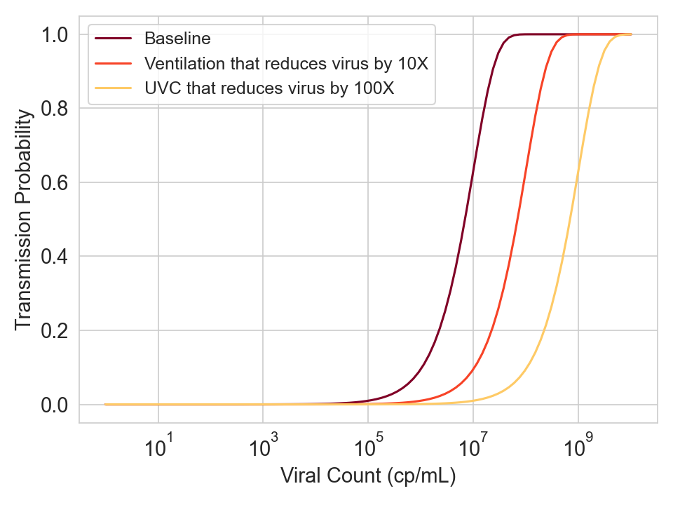
Figure 6. Hypothetical curves for three different conditions.
So once we have completed this experiment, we don’t need to repeat it for other types of interventions on human recipients. We just need to measure the reduction in virus concentration in the air during whatever intervention we want to test, which will be proportional to the reduction in \(\beta\).
To a lesser extent, we can even generalize to other viruses, which is nice since it allows you to run this experiment on the common cold. Because \(\lambda\) is proportional to a virus-specific baseline susceptibility constant and air quality constants, you’ll know that if an air quality intervention shifts the curve for the common cold by K log units, then it should also shift the curve for the other virus by K log units. This is true even if the other virus has a flatter curve due to higher variance in baseline susceptibility (see code). The only limitation is that if you want to quantify the aggregate reduction in infections, you’ll still need to measure the dose-response curve for the other virus once and then integrate over the distribution of viral counts.
Summary
If anyone has $10 million lying around and is able to run this experiment and model it correctly, you will:
- Conclusively establish the viral counts at which people become meaningfully infectious with the virus you’re testing
- Conclusively establish the effectiveness of your intervention, convincing experts and laypeople alike
- Generalize these results to other interventions, without needing to infect anyone else.
- Partially generalize these results to other viruses
Footnote
\(^1\)To a first approximation, viral RNA count is proportional to infectious virus count and claims otherwise have been overstated. See the “Live virus count is mostly proportional to RNA count” section of this post for evidence.