You’re probably measuring your treatment effect incorrectly
28 Mar 2021A special thanks to Scott Cunningham and Dean Eckles for helping me clear up my own confusion and inspiring me to write this blog post, and to Scott for his excellent book, which taught me a lot of background for this.
You’ve developed a new health program and you want to measure its impact. You run a randomized experiment where half of participants are allowed to get treatment, and half are not. Of those allowed to get treatment, 80% actually choose to get treated.
You would like to report the answer to a very basic question: How much did the treatment help the people who got treated? You might think that’s a simple question to answer. But you’d be wrong.
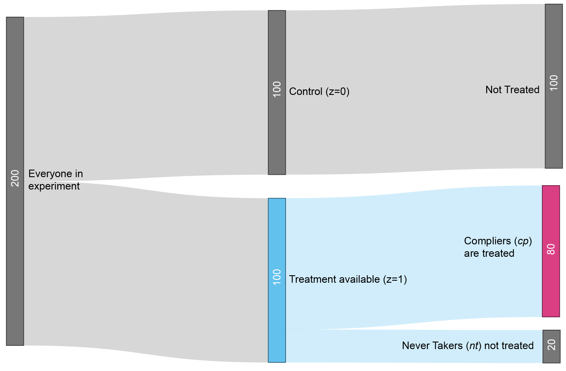
Figure 1: Experiment flowchart. The participants in the treatment group who actually take the treatment are called “compliers” (cp). The participants who don’t are called “never takers” (nt).
Before getting started, I know many readers might wish to suggest a different question: What was the impact of making the treatment available, regardless of whether the eligible users got treated? That’s an important question that we’ll get to later. For now, let’s focus on the impact to those who actually got treated. There’s a few ways you might think this could be answered, but most of them are wrong.
Wrong approach #1
Suppose you are measuring a health score. One idea is to compute the difference between the average outcome in the treated subset and the average outcome in the control group.
\[Y_{cp, z=1} - Y_{z=0}\]Here, \(Y\) represents the average within a group, \(z\) represents assignment to treatment availability, and \(cp\) is shorthand for complier, referring to people who complied with the instructions. \(Y_{cp,z=1}\) therefore represents the group that actually received treatment, since they were compliers (\(cp\)) who were randomly assigned to treatment availability (\(z=1\)). The other term \(Y_{z=0}\), represents the control group (\(z=0\)). In this type of analysis, we ignore the group of people who refused treatment.
This approach has a bad selection bias problem. Compliers may comply because they have poorer health to begin with. Suppose the average health score in the overall population is \(Y=50\), and that compliers start out with score of \(Y_{cp,z=1} = 40\). Even even if the treatment improves the health of the compliers by, say, \(4\) points, they will still end up with lower health (\(44\)) than the control group. This analysis could make a useful treatment look like it was harming people’s health!
Wrong approach #2
To correct for baseline differences, my natural inclination is to compute the post-treatment vs pre-treatment difference for the treated compliers, and then compare that difference to the same post- vs pre- difference for the control group. This aproach, which is called Differences-in-Differences (DD), estimates the treatment effect for compliers as
\[(Y_{cp, z=1} - Y_{cp, z=1,pre}) - (Y_{z=0} - Y_{z=0,pre})\]where \(Y_{cp, z=1}\) is the post-treatment health of the treated compliers and \(Y_{cp, z=1,pre}\) is their pre-treatment health.
Figure 2 shows how this works. Upon taking the treatment, the health of the treated compliers declines slower than the health of the control group. By the logic of DD, the treatment must have helped the compliers, since otherwise their health would have been poorer. This counterfactual health of the compliers, were they not to be treated, is denoted by \(Y_{cp, z=1}^0\) where the superscript indicates a counterfactual world where they are not treated.
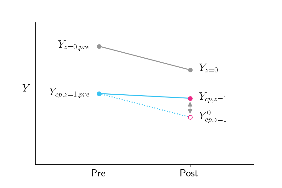
Figure 2: Pre-treatment and post-treatment health scores for the control group (gray line) and the treated compliers (solid blue line). The pink open circle represents the score the treated compliers would have gotten if they did not receive treatment, assuming they would have had the same slope as the control group.
DD attempts to estimate \(Y_{cp, z=1}^0\) by assuming the treated compliers would have had the same slope as the control group, in the counterfactual world where they didn’t get treated. But that’s not a safe assumption! It is completely conceivable that the compliers, were they not treated, would have a different slope than the control group.
Figure 3 shows this in action, where \(Y_{cp, z=1}^0\) is lower than assumed by the parallel slopes assumption of Figure 2. Were \(Y_{cp, z=1}^0\) to be as shown in Figure 3, the DD approach would underestimate the impact of treatment on compliers.
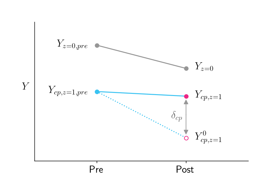
Figure 3: Similar to Figure 2 except that the counterfactual outcome in the bottom right is lower than in Figure 2, which assumed parallel slopes to the control group.
Correct approach: Instrumental Variables and the Local Average Treatment Effect
DD is a reasonable approach in situations where there is no randomization. But because our experiment is randomized, there is a clever trick we can use to get a much better estimate.
The parameter we ultimately want to estimate is \(\delta_{cp}\), which is the difference between the treated compliers’ outcome and their counterfactual outcome if they didn’t receive treatment, as shown in Figure 3.
\[\delta_{cp}=Y_{cp, z=1} - Y_{cp, z=1}^0\]This value is called the Local Average Treatment Effect (LATE), since it reflects the impact of the treatment on a particular subpopulation.
To compute the LATE we only need to know two numbers: \(Y_{cp, z=1}\) and \(Y_{cp, z=1}^0\). It’s easy to get \(Y_{cp, z=1}\). That’s just the actual outcome of the treated compliers. But how could we possibly know the counterfactual \(Y_{cp, z=1}^0\)? The DD approach attempted to estimate it with some flawed assumptions, but how can we possibly do better than that?
Remarkably, there is a great way to estimate \(Y_{cp, z=1}^0\) without relying on the flawed assumptions of DD! Here’s the trick, which is based on the the logic of instrumental variables: Because of randomization, we should expect the control group’s outcomes to be the same as the treatment-available group’s outcomes in the counterfactual world where no one got treated.
\[Y_{z=0} = Y_{z=1}^0\]The treatment-available group is composed of two subgroups, compliers (cp) and never-takers (nt). \(Y_{z=1}^0\) is therefore a weighted average of these two groups, which we can substitute into the formula above
\[Y_{z=0} = \pi_{cp} Y_{cp, z=1}^0 + \pi_{nt} Y_{nt, z=1}\]where \(\pi_{cp}\) is the fraction of compliers and \(\pi_{nt}\) is the fraction of never-takers. We do not place a superscript on \(Y_{nt, z=1}\) since it represents the realized (i.e. not counterfactual) world where never-takers did not receive treatment. We can now solve for \(Y_{cp, z=1}^0\), since everything else in the equation is already known.
\[Y_{cp, z=1}^0 = \frac{Y_{z=0} - \pi_{nt} Y_{nt, z=1}}{\pi_{cp}}\]Ultimately our goal is to estimate \(\delta_{cp} = Y_{cp, z=1} - Y_{cp, z=1}^0\), so substituting we have:
\[\delta_{cp} = Y_{cp, z=1} - \frac{Y_{z=0} - \pi_{nt} Y_{nt, z=1}}{\pi_{cp}}\]Further rearrangement gives us
\[\delta_{cp} = \frac{Y_{z=1} - Y_{z=0}}{\pi_{cp}}\]This is a remarkably simple formula. The impact on treated compliers is just the difference between the treatment group and control group, divided by the fraction of compliers. Even more remarkable is that this formula was only discovered recently.
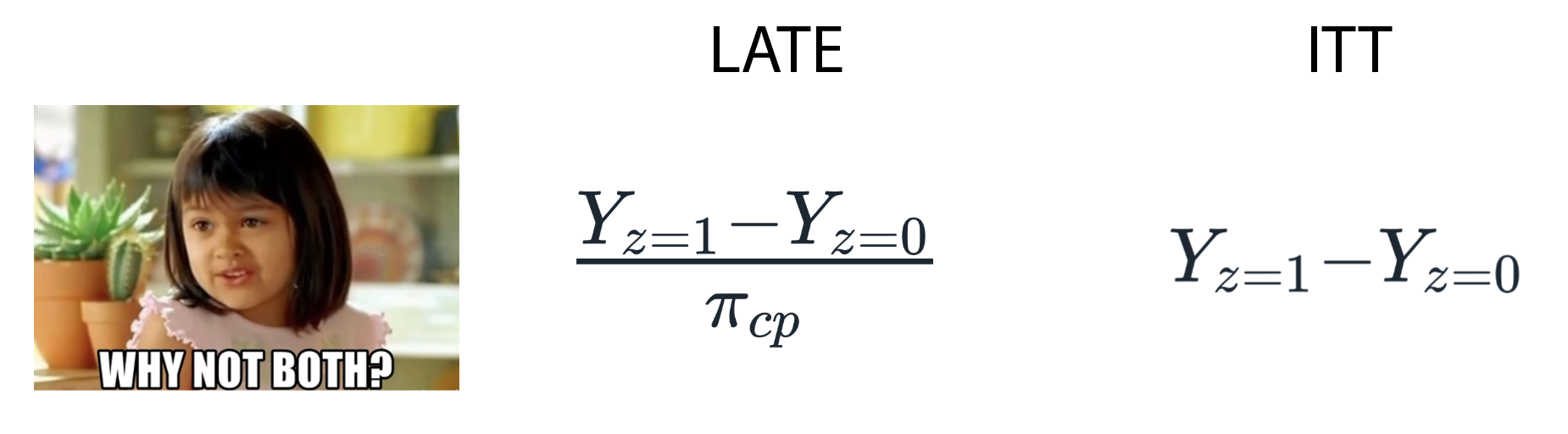
To help us summarize this, let’s hand it over to Drake.
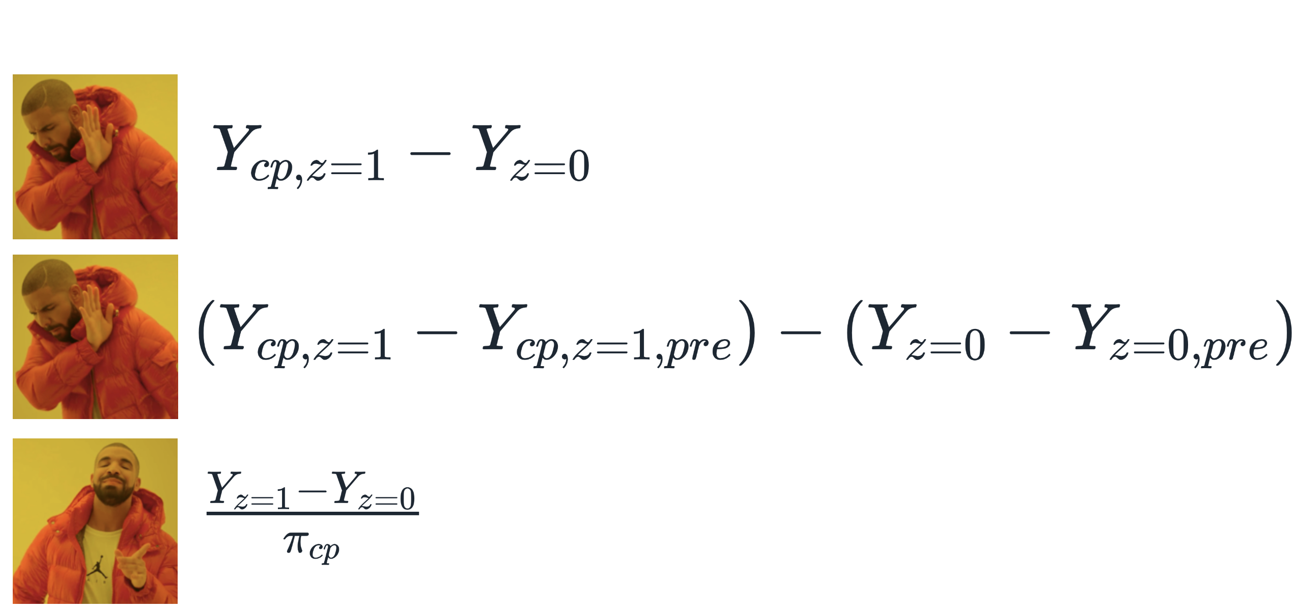
Figure 4: Summary of methods for estimating the LATE in a randomized experiment with partial compliance.
Additional comments
Complier biases that LATE does and does not account for
The LATE tells you how much the treatment affects the people who actually got treated. This group of people is biased in two ways, and LATE only accounts for one of these biases. The first bias is that this group’s counterfactual outcomes might be different from other groups. LATE accounts for that by correctly reporting the impact of the treatment relative to the counterfactual. The second bias is that the treatment might be more effective in the complier group than in the never-taker group. That bias is unescapable and is known as a heterogenous treatment effect. The way to deal with this bias is to acknowledge it transparently.
LATE and Intention To Treat
The fact that the treatment may have a different effect in the treated compliers is one limitation of LATE. But there are a couple other limitations as well. One is that LATE doesn’t tell you about the overall impact of your policy. If only 10% of people in the treatment group actually choose to take the treatment, the overall impact of your policy might be small, and you might want to consider treatments with higher uptake. The other limitation is that in many medical applications, the treatment involves more than a single dose, and people can withdraw midway through the program. This means that the distinction between complier and never-taker can be strongly driven by the effectiveness of the treatment, making the LATE a less generalizable metric. For these reasons, researchers often report the Intention To Treat (ITT) metric, which is the impact of being assigned to treatment (\(Y_{z=1} - Y_{z=0})\) rather than the impact of being treated. While suffering from its own limitations, ITT should always be reported, often as the headline metric. Nevertheless, for many applications, particularly those involving one-time enrollments, the LATE is a critical and complementary metric, and one that’s trickier – and yet in some ways simpler – than I ever imagined.