Instrumental variables analysis for non-economists

Instrumental Variables estimation is one of the most popular techniques in causal inference. But it can be a little hard to understand, especially when it is presented with terms mostly familiar to economists, such as “endogeneity” and “correlated with the error term”. In this blog post, I share some visualizations that gave me better intuitions about it. The post is designed for scientists and engineers who are familiar with causal inference, but who have a visual way of thinking that differs from how economists think.

Imagine that you have a treatment variable \(D\) that causes an outcome \(Y\). The true data-generating process is

where \(\delta\) is the average treatment effect and \(\varepsilon\) is some error. \(Y\), \(D\), and \(\varepsilon\) are vectors and \(\delta\) is scalar.

The causal graph is shown below. Whereas the equation above puts outcome \(Y\) on the left side, causal graphs typically put the outcome \(Y\) on the right side. The graph shows simulated data for 16 units, each represented by a bar. The height of each bar represents the value for that unit and that variable. The treatment variable \(D\) takes on continuous values, and the outcome \(Y\) is decomposed into its two components, \(D\) and its own error.

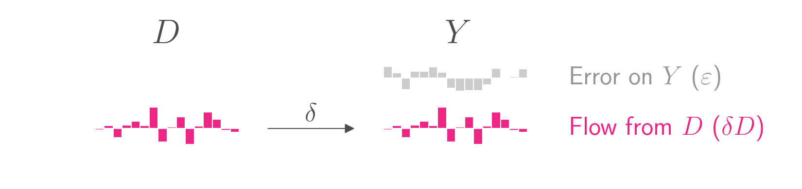
To keep the figures clean, I have set \(\delta\) to 1, a practice I will continue with all coefficients throughout this blog post. Just keep in mind that in almost all real world cases, the coefficients will not be 1.

Anyway, the goal of causal inference is to estimate the treatment effect \(\delta\). If your causal graph is as simple as the one above, you’re in luck. All you need to do is regress \(Y\) on \(D\). The coefficient on \(D\) in that regression will be an unbiased estimate of \(\delta\), which is the parameter you want to estimate.

Unfortunately, most causal graphs aren’t so simple. Often there is an unobserved confounder, \(U\), which contributes to both \(D\) and \(Y\). For example, if you want to measure the impact of smoking \(D\) on lung cancer \(Y\), you might want to consider the possibility that certain unobserved genetic factors \(U\) might cause both smoking and lung cancer.

The data-generating model is as follows.

The causal graph is shown below.

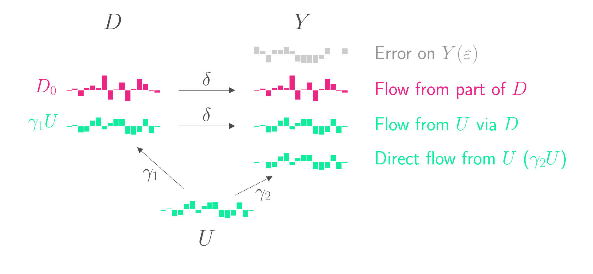
\(U\) affects \(D\), which then goes on to affect \(Y\). But \(U\) also directly affects \(Y\). This is confounding. A naive regression of \(Y\) on \(D\) will overestimate \(\delta\). That’s because part of the relationship between \(D\) and \(Y\) isn’t due to \(D\)’s causal impact on \(Y\).

If \(U\) was observable, you could include it as a covariate in your regression. But since \(U\) is unobservable, you don’t have that option.

This is where instrumental variables come in.

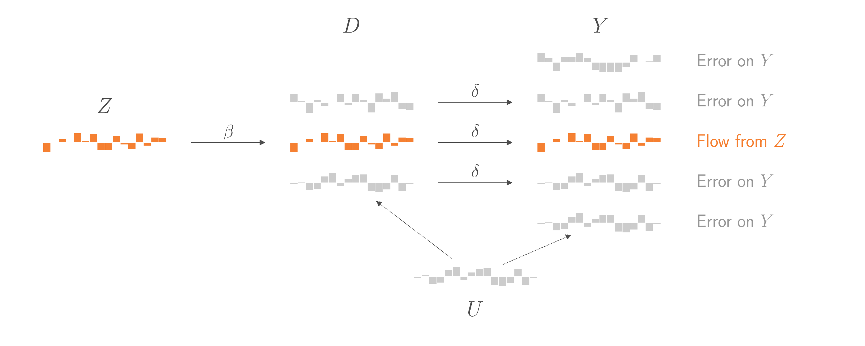
An instrumental variable \(Z\) is a variable that has some effect on \(D\), but has no other relation to \(Y\), except through \(D\). In the case of smoking (\(D\)) and lung cancer (\(Y\)), a good instrumental variable might be a cigarette tax (\(Z\)), which might vary from state to state. The cigarette tax will affect smoking, and should have no other relation to lung cancer except through smoking.

The graph below introduces the instrumental variable \(Z\). This new display also splits the previously pink component into two components. The first component (in orange) comes from \(Z\)’s impact on \(D\). The second component (in blue) is random error in \(D\) that is not explained by either \(Z\) or \(U\).

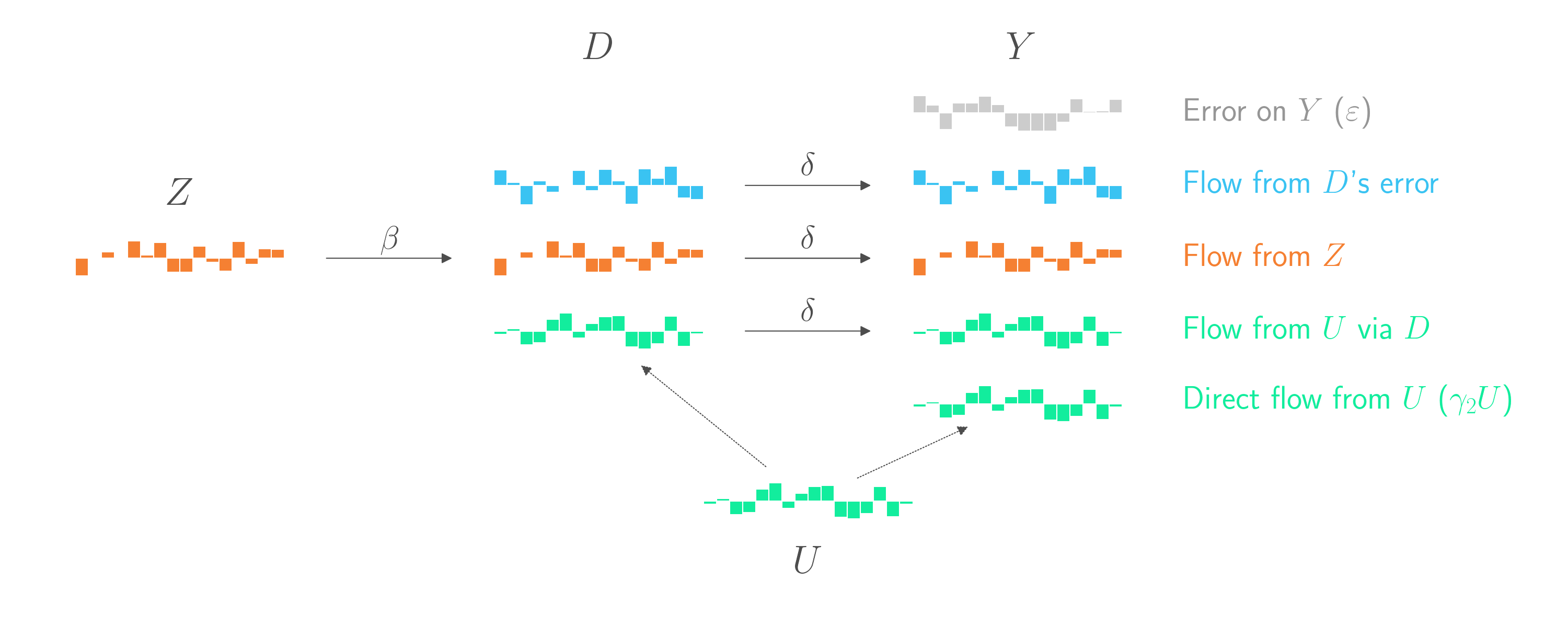
This gives us an opportunity! The part of \(D\) that is controlled by \(Z\) are effectively random, quasi-exerimental changes to \(D\) that are independent of \(U\). Let’s (generously) call that part \(\hat{D}\). If we could regress \(Y\) on \(\hat{D}\), we’d have a chance to use the straightforward regression technique from the start of this blog post. Everything else in \(Y\) that didn’t come from \(\hat{D}\) would just be error, and it wouldn’t matter if some of that error comes from \(U\). As in the example at the start of this blog post, the coefficient on \(\hat{D}\) would be an unbiased estimate of \(\delta\). And by assumption, that \(\delta\) is the same \(\delta\) that connects \(D\) overall to \(Y\). And that’s what we ultimately want to estimate.

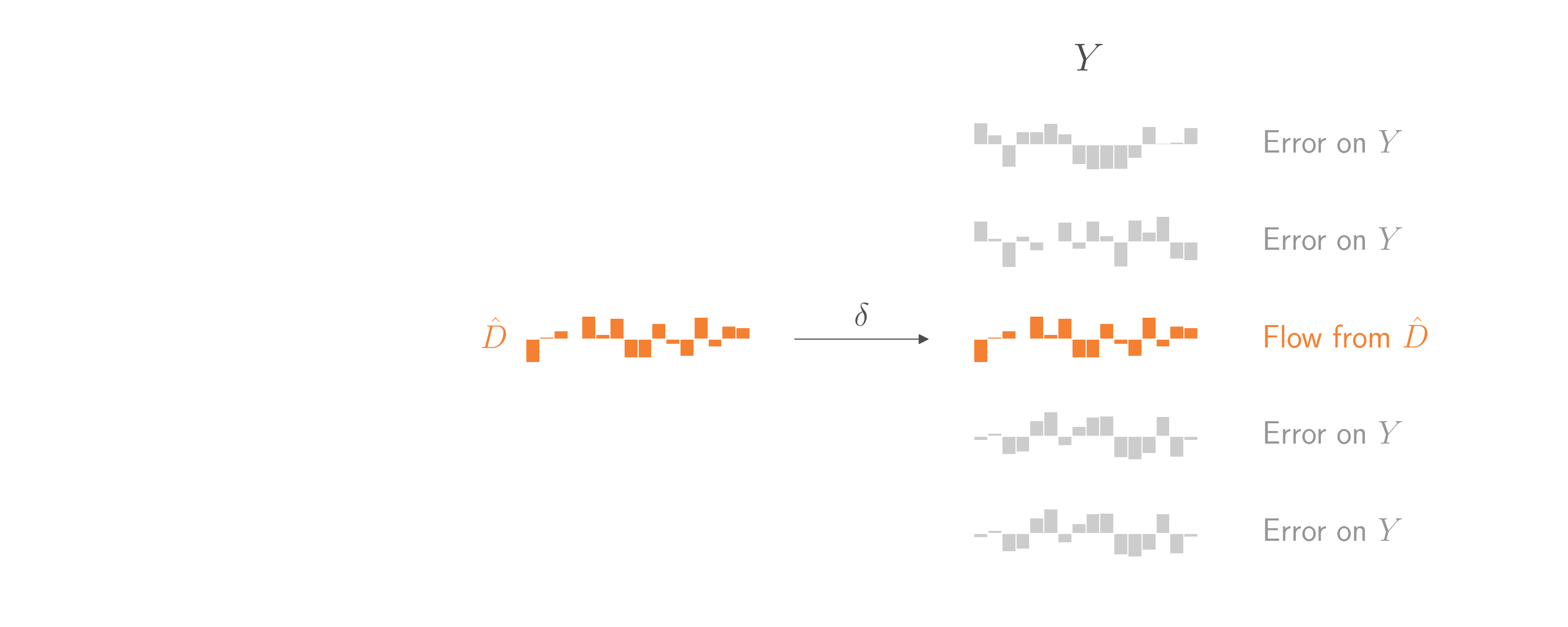
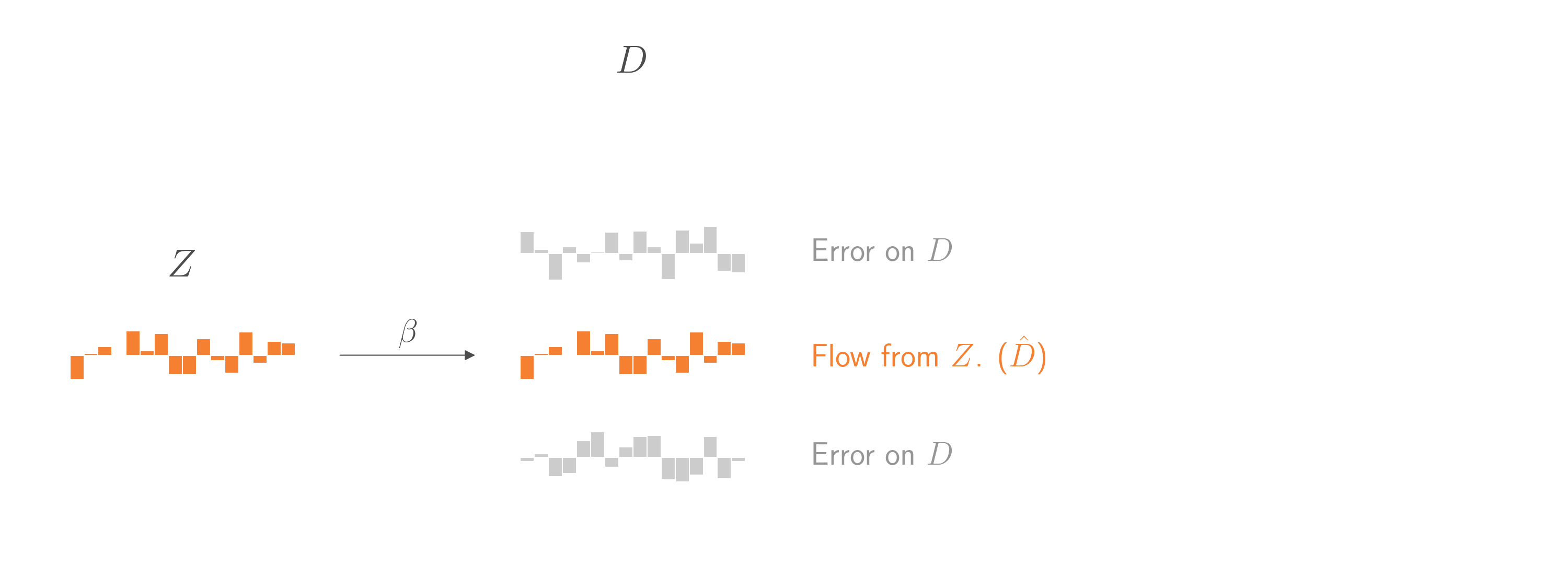
That would be nice. But how can we isolate \(\hat{D}\)? By regressing \(D\) on \(Z\)! Using the same logic, regressing \(D\) on \(Z\) will treat everything in \(D\) that doesn’t come from \(Z\) as error. The coefficient relating \(Z\) to \(D\) will be an unbiased estimate of the causal weight \(\beta\) that relates \(Z\) to \(D\). Critically, the predictions from that regression model will almost exactly estimate the component in \(D\) that comes from \(Z\). (Well, there’s some bias from overfitting, but that can wait for another blog post.)

Putting it all together, to estimate \(\delta\) we need to avoid any part of \(D\) that comes from \(U\), since \(U\) is an unobservable confound. Fortunately, there is a part of \(D\) that we can isolate. It’s the part that comes from \(Z\), and we call it \(\hat{D}\). To isolate \(\hat{D}\), we regress \(D\) on \(Z\) and then use the model to make a prediction from input \(Z\). Once we have \(\hat{D}\), we can regress \(Y\) on \(\hat{D}\) to estimate \(\delta\). By assumption, this \(\delta\) is the same \(\delta\) that comes from the other parts of \(D\), and is therefore the average treatment effect we want to estimate. (Note: This approach, called Two-Stage Least Squares, will underestimate the standard errors on \(\delta\).)

In Python:

from numpy.random import randn
from sklearn.linear_model import LinearRegression

# Generate data from true model 
n = 10000
delta = 1.3
beta = 1.5
gamma_1 = 1.7 # weight from U to d
gamma_2 = 1.7 # weight from U to y
z = randn(n, 1)
u = randn(n, 1)
d = beta * z + gamma_1 * u + randn(n, 1)
y = delta * d + gamma_2 * u + randn(n, 1)

# Naive regression (bad)
mod0 = LinearRegression()
mod0.fit(d, y)
print(mod0.coef_) # Will be too high

# First stage regression in IV approach
mod1 = LinearRegression()
mod1.fit(z, d)
d_hat = mod1.predict(z)

# Second stage regression in IV approach
mod2 = LinearRegression()
mod2.fit(d_hat, y)
print(mod2.coef_) # Unbiased estimate of delta

Of course, our assumptions might not always hold. For example, many instruments might be related to the outcome variable in ways not shown in these graphs. In the case of smoking, there might be correlations between cigarette taxes and lung cancer that aren’t causally mediated by smoking. Often you can control for this. For example, if some observable variable \(X\) points to \(Z\), \(D\), and \(Y\), you can just include it as covariate in your two regressions. Doing so will block the nondirect paths from \(Z\) to \(Y\).

We also assumed that each component of \(D\) will share the same impact \(\delta\) on \(Y\). That assumption won’t always be true. Perhaps people whose smoking behavior is sensitive to a tax may have a different \(\delta\) than other people. When that happens, you may still be able to estimate \(\delta\) for a subset of the population (or more precisely, a weighted average of subsets), but you won’t be able to generalize it to everyone.