Things that confused me about cross-entropy

26 Dec 2020

Every once in a while, I try to better understand cross-entropy by skimming over some Medium posts and StackExchange answers. I always come away only half-understanding it.

A major cause of confusion is that different sources use different notations and conventions. Here are some that tripped me up.

p and q vs y and p

In information theory, the cross-entropy for an event with \(M\) discrete outcome classes is

\[H(p, q) = -\sum_{j=1}^M{p_j log (q_j)}\]

… where \(p\) is the true distribution of outcomes and \(q\) is the approximating distribution.

But in machine learning, the cross-entropy is defined as:

\[H(y, p) = -\sum_{j=1}^M{y_j log (p(y_j))}\]

… where \(y\) are the true labels and \(p(y)\) is the approximating distribution, i.e. the classifier’s probability predictions.

Notice that the meaning of \(p\) has been reversed! In information theory, it is the true distribution. In machine learning, it is the approximating distribution.

This points to a key difference between generic information theory and machine learning applications. In information theory, the target distribution \(p\) is a probability distribution where the probability mass can be distributed broadly over the classes. In machine learning, the target distribution \(y\) has all of its mass allocated to a known label.

Multiple classes vs multiple events, and indicators vs labels

As shown above, the cross-entropy for a single event with \(M\) classes is:

\[H(y, p) = -\sum_{j=1}^M{y_j log (p(y_j))}\]

If there are multiple events, you just need to sum up the cross-entropies from all the events so that the total cross-entropy is:

\[H(y, p) = -\sum_{i=1}^N \sum_{j=1}^M{y_j^{(i)} log (p(y_j^{(i)}))}\]

… where \(N\) is the number of events.

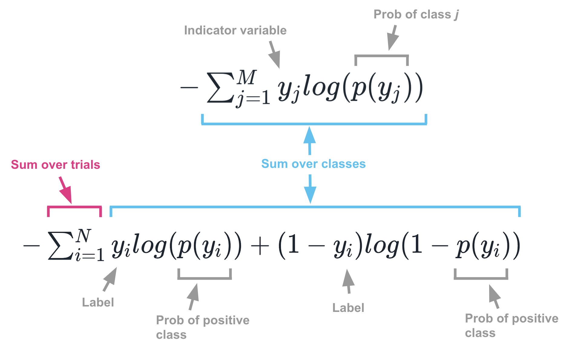
This all makes notational sense. Unfortunately, confusion arises when people use non-compact notation for summing over binary classes. When dealing with binary classification, it’s common to see cross-entropy defined as:

\[H(y, p) = -\sum_{i=1}^N{y_i log (p(y_i)) + (1-y_i) log (1 -p(y_i))}\]

Superficially, this looks a lot like the first formula, but it’s actually just a clever and somewhat confusing way of writing the second formula for binary classes. Its notation differs from previous formulas in a few ways:

• First, this formula sums over events, whereas the first formula in this section only sums over classes.
• Second, because it is summing over events, it uses \(p(y_i)\) rather than \(p(y_j)\). Here, \(p(y_i)\) refers to the probability of a positive result on an event. In previous formulas, \(p(y_j)\) referred to the probability of the particular class being considered in the summation loop for that event.
• Third, it’s easier to think of \(y_i\) (when not wrapped by a \(p\)) as a label, rather than an indicator variable. When the event has an outcome of 1, \(y_i\) is 1. When it has an outcome of 0, \(y_i\) is 0. In previous formulas, as you loop through classes you would set \(y_j\) to be 1 whenever the outcome was the class being considered; otherwise you set it to 0.

The image below summarizes the many confusing differences between these formulas.

Where to learn about cross-entropy

I don’t know if there is a single best place to learn about cross-entropy, but below are a few places that were helpful. If you read them make sure you think about (a) how they are notating the true distribution and the approximating distribution (b) whether they are writing about single events or multiple events (c) whether they are writing about binary classes or multi classes and (d) whether the \(y\)’s are indicators or labels.

• Statistical Rethinking. Information theory notation, single event case, multiple classes.
• Andrew Webb. Both notations, both the single and multiple event case, multiple classes.
• Harshith. ML notation, multiple events, binary classes.