
Empirical Bayes for multiple sample sizes
03 May 2017Here’s a data problem I encounter all the time. Let’s say I’m running a website where users can submit movie ratings on a continuous 1-10 scale. For the sake of argument, let’s say that the users who rate each movie are an unbiased random sample from the population of users. I’d like to compute the average rating for each movie so that I can create a ranked list of the best movies.
Take a look at my data:
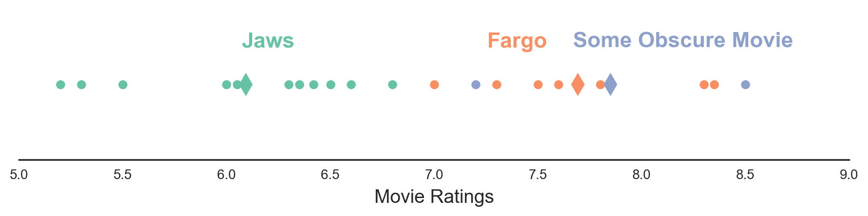
Figure 1. Each circle represents a movie rating by a user. Diamonds represent sample means for each movie.
I’ve got two big problems here. First, nobody is using my website. And second, I’m not sure if I can trust these averages. The movie at the top of the rankings was only rated by two users, and I’ve never even heard of it! Maybe the movie really is good. But maybe it just got lucky. Maybe just by chance, the two users who gave it ratings happened to be the users who liked it to an unusual extent. It would be great if there were a way to adjust for this.
In particular, I would like a method that will give me an estimate closer to the movie’s true mean (i.e. the mean rating it would get if an infinite number of users rated it). Intuitively, movies with mean ratings at the extremes should be nudged, or “shrunk”, towards the center. And intuitively, movies with low sample sizes should be shrunk more than the movies with large sample sizes.
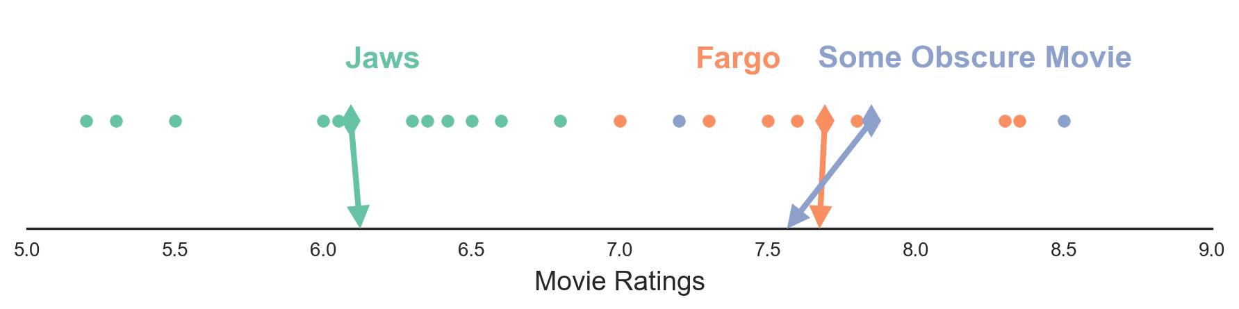
Figure 2. Each circle represents a movie rating by a user. Diamonds represent sample means for each movie. Arrows point towards shrunken estimates of each movie’s mean rating. Shrunken estimates are obtained using the MSS James-Stein Estimator, described in more detail below.
As common a problem as this is, there aren’t a lot of accessible resources describing how to solve it. There are tons of excellent blog posts about the Beta distribution, which is useful if you wish to estimate the true fraction of an occurrence among some events. This works well in the case of Rotten Tomatoes, where one might want to know the true fraction of “thumbs up” judgments. But in my case, I’m dealing with a continuous 1-10 scale, not thumbs up / thumbs down judgments. The Beta-binomial distribution will be of little use.
Many resources mention the James-Stein Estimator, which provides a way to shrink the mean estimates only when the variances of those means can be assumed to be equal. That assumption usually only holds when the sample sizes of each group are equal. But in most real world examples, the sample sizes (and thus the variances of the means) are not equal. When that happens, it’s a lot less clear what to do.
After doing a lot of digging and asking some very helpful folks on Twitter, I found several solutions. For many of the solutions, I ran simulations to determine which worked best. This blog post is my attempt to summarize what I learned. Along the way, we’ll cover the original James-Stein Estimator, two extensions to the James-Stein Estimator, Markov Chain Monte Carlo (MCMC) methods, and several other strategies.
Before diving in, I want to include a list of symbol definitions I’ll be using because – side rant – it sure would be great if all stats papers did this, given that literally every paper I read used its own idiosyncratic notations! I’ll define everything again in the text, but this is just here for reference:
| Symbol | Definition |
| \(k\) | The number of groups. |
| \(\theta_i\) | The true mean of a group. |
| \(x_i\) | The sample mean of a group. The MLE estimate of \(\theta_i\). |
| \(\epsilon^{2}_i\) | The true variance of observations within a group. |
| \(\epsilon^2\) | The true variance of observations within a group if we assume all groups have the same variance. |
| \(s^{2}_i\) | The sample variance of a group. The MLE estimate of \(\epsilon^{2}_i\). |
| \(n_i\) | The number of observations in a group. |
| \(n\) | The number of observations in a group, if we assume all groups have the same size. |
| \(\sigma^{2}_i\) | The true variance of a group’s mean. If each group has the same variance of observations, then \(\sigma^{2}_i = \epsilon^{2} / n_i\). If each group has different variances of observations, then \(\sigma^{2}_i = \epsilon^{2}_i / n_i\). |
| \(\sigma^{2}\) | Like \(\sigma^{2}_i\), but if we assume all groups had the same variance of the mean. Equal to \(\epsilon^{2} / n\). |
| \(\hat{\sigma^{2}_i}\) | Estimate of \(\sigma^{2}_i\). |
| \(\hat{\sigma^{2}}\) | Estimate of \(\sigma^{2}\). |
| \(\mu\) | The true mean of the \(\theta_i\)’s (the true group means). The mean of the distribution from which the \(\theta_i\)’s are drawn. |
| \(\overline{X}\) | The sample mean of the sample means. |
| \(\tau^{2}\) | The true variance of the \(\theta_i\)’s (the true group means). The variance of the distribution from which the \(\theta_i\)’s are drawn. |
| \(\hat{\tau^{2}}\) | Estimate of \(\tau^{2}\). |
| \(\hat{B}\) | Estimate of the best term for weighting \(x_i\) and \(\overline{X}\) when calculating \(\hat{\theta_i}\). Assumes each group has the same \(\sigma^2\). |
| \(\hat{B_i}\) | Estimate of the best term for weighting \(x_i\) and \(\overline{X}\) when calculating \(\hat{\theta_i}\). Does not assume that all group’s have the same \(\sigma^{2}_i\). |
| \(\hat{\theta_i}\) | Estimate of a true group means. Its value depends on the method we use. |
| \(k_{\Gamma}\) | Shape parameter for the Gamma distribution from which sample sizes are drawn. |
| \(\theta_{\Gamma}\) | Scale parameter for the Gamma distribution from which sample sizes are drawn. |
| \(\mu_v\) | In simulations in which group observation variances \(\epsilon^{2}_i\) are allowed to vary, this is the mean parameter of the log-normal distribution from which the \(\epsilon^{2}_i\)’s are drawn. |
| \(\tau^{2}_v\) | In simulations in which group observation variances \(\epsilon^{2}_i\) are allowed to vary, this is the variance parameter of the log-normal distribution from which the \(\epsilon^{2}_i\)’s are drawn. |
Quick Analytic Solutions
Our goal is to find a better way of estimating \(\theta_i\), the true mean of a group. A common theme in many of the papers I read is that good estimates of \(\theta_i\) are usually weighted averages of the group’s sample mean \(x_i\) and the global mean of all group means \(\overline{X}\). Let’s call this weighting factor \(\hat{B_i}\).
\[\hat{\theta_i} = \left(1-\hat{B_i}\right) x_i + \hat{B_i} \overline{X}\]This seems very sensible. We want something that is in between the sample mean (which is probably too extreme) and the mean of means. But how do we know what value to use for \(\hat{B_i}\)? Different methods exist, and each leads to different results.
Let’s start by defining \(\sigma^{2}_i\), the true variance of a group’s mean. This is equivalent to \(\epsilon^{2}_i / n_i\), where \(\epsilon^{2}_i\) is the true variance of the observations within that group, and \(n_i\) is the sample size of the group. According to the original James-Stein approach, if we assume that all the group means have the same known variance \(\hat{\sigma^2}\), which would usually only happen if the groups all had the same sample size, then we can define a common \(\hat{B}\) for all groups as:
\[\hat{B} = \frac{\left(k-3\right)\hat{\sigma^2}}{\sum{(x_i - \overline{X})^2}}\]This formula seems really weird and arbitrary, but it begins to make more sense if we rearrange it a bit and sweep that pesky \(\left(k-3\right)\) under the rug and replace it with a \((k-1)\). Sorry hardliners!
\[\begin{eqnarray} \hat{B} &\approx& \frac{\left(k-1\right)\hat{\sigma^2}}{\sum{(x_i - \overline{X})^2}}\\ \\ &=& \frac{\hat{\sigma^2}}{\sum{(x_i - \overline{X})^2}/\left(k-1\right)} \\ \\ &=& \frac{\hat{\sigma^2}}{\hat{\tau^{2}} + \hat{\sigma^2}} \end{eqnarray}\]Before getting to why this makes sense, I should explain the last step above. The denominator \(\sum{(x_i - \overline{X})^2}/\left(k-1\right)\) is the observed variance of the observed sample means. This variance comes from two sources: \(\tau^2\) is the true variance in the true means and \(\sigma^2\) is the true variance caused by the fact that each \(x_i\) is computed from a sample. Since variances add, the total variance of the observed means is \(\tau^{2} + \sigma^{2}\).
Anyway, back to the result. This result is actually pretty neat. When we estimate a \(\theta_i\), the weight that we place on the global mean \(\overline{X}\) is the fraction of total variance in the means that is caused by within-group sampling variance. In other words, when the sample mean comes with high uncertainty, we should weight the global mean more. When the sample mean comes with low uncertainty, we should weight the global mean less. At least directionally, this formula makes sense. Later in this blog post, we’ll see how it falls naturally out of Bayes Law.
The James-Stein Estimator is so widely applicable that many other fields have discovered it independently. In the image processing literature, it is a special case of the Wiener Filter, assuming that both the signal and the additive noise are Gaussian. In the insurance world, actuaries call it the Bühlmann model. And in animal breeding, early researchers called it the Best Unbiased Linear Prediction or BLUP (technically the Empirical BLUP). The BLUP approach is so useful, in fact, that it has received the highly coveted endorsement of the National Swine Improvement Federation.
While the original James-Stein formula is useful, the big limitation is that it only works when we believe that all groups have the same \(\sigma^2\). In cases where we have different sample sizes, each group will have it’s own \(\sigma^{2}_i\). (Recall that \(\sigma^{2}_i = \epsilon^{2}_i / n_i\).) We’re going to want to shrink some groups more than others, and the original James-Stein estimator does not allow this. In the following sections, we’ll look at a couple of extensions to the James-Stein estimator. These extensions have analogues in the Bühlmann model and BLUP literature.
The Multi Sample Size James-Stein Estimator
The most natural extension of James-Stein is to define each group’s \(\hat{\sigma^{2}_i}\) as the squared standard error of the group’s mean. This allows us to estimate a weighting factor \(\hat{B_i}\) tailored to each group. Let’s call this the Multi Sample Size James-Stein Estimator, or MSS James-Stein Estimator.
\[\hat{B_i} = \frac{\hat{\sigma^{2}_i}}{\hat{\tau^{2}} + \hat{\sigma^{2}_i}}\]The denominator can just be estimated as the variance across group sample means.
As reasonable as this approach sounds, it somehow didn’t feel totally kosher to me. But when I looked into the literature, it seems like most researchers basically said “yup, that sounds pretty reasonable”.
To test this approach, I ran some simulations on 1000 artificial datasets. Each dataset involved 25 groups with sample sizes drawn from a Gamma distribution \(\Gamma(k_{\Gamma}=1.5,\theta_{\Gamma}=10)\). True group means (\(\theta_i\)’s) were sampled from a Normal distribution \(\mathcal{N}(\mu, \tau^2)\). Observations within each group were sampled from \(\mathcal{N}(\theta_i, \epsilon^2)\), where \(\epsilon\) was shared between groups.
For each dataset I computed the Mean Squared Error (MSE) between the vector of true group means and the vector of estimated group means. I then averaged the MSEs across datasets. This process was repeated for a variety of different values of \(\epsilon\) and for two different estimators: The MSS James-Stein Estimator and the Maximum Likelihood Estimator (MLE). To compute the MLE, I just used \(x_i\) as my \(\hat{\theta_i}\) estimate.
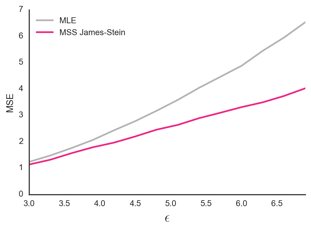
Figure 3. Mean Squared Error between true group means and estimated group means. In this simulation, the \(\epsilon\) parameter for within-group variance of observations is shared by all groups.
As expected, the MSS James-Stein Estimator outperformed the MLE, with lower MSEs particularly for high values of \(\epsilon\). This make sense. When the raw sample means are noisy, the MLE should be especially untrustworthy and it makes sense to pull extreme estimates back towards the global mean.
The Multi Sample Size Pooled James-Stein Estimator
One thing that’s a little weird about the MSS James-Stein Estimator is that even though we know all the groups should have the same within-group variance \(\epsilon^2\), we still estimate each group’s standard error separately. Given what we know, it might make more sense to pool the data from all groups to estimate a common \(\epsilon^2\). Then we can estimate each group’s \(\sigma^{2}_i\) as \(\epsilon^2 / n_i\). Let’s call this approach the MSS Pooled James-Stein Estimator.
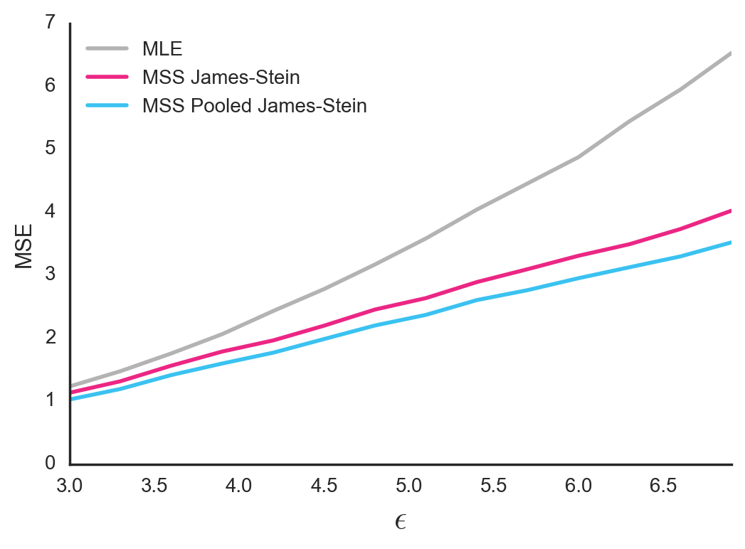
Figure 4. Mean Squared Error between true group means and estimated group means. In this simulation, the \(\epsilon\) parameter for within-group variance of observations is shared by all groups.
This works a bit better. By obtaining more accurate estimates of each group’s \(\sigma^{2}_i\), we are able to find a more appropriate shrinking factor \(B_i\) for each group.
Of course, this only works better because we created the simulation data in such a way that all groups have the same \(\epsilon^2\). But if we run a different set of simulations, in which each group’s \(\epsilon_i\) is drawn from a log-normal distribution \(ln\mathcal{N}\left(\mu_v, \tau^{2}_v\right)\), we obtain the reverse results. The MSS James-Stein Estimator, which estimates a separate \(\hat{\epsilon^{2}_i}\) for each group, does a better job than the MSS Pooled James-Stein Estimator. This makes sense.
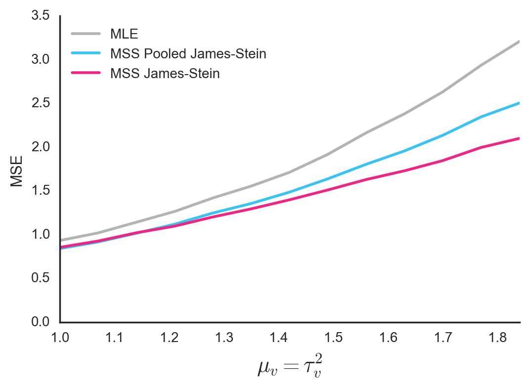
Figure 5. Mean Squared Error between true group means and estimated group means. In this simulation, each group has its own variance parameter \(\epsilon^2\) for the observations within the group. These parameters are sampled from a log-normal distribution \(ln\mathcal{N}\left(\mu_v, \tau^{2}_v\right)\). For simplicity, the two parameters of this distribution are always set to be identical, and are shown on the horizontal axis.
Which method you choose should depend on whether you think your groups have similar or different variances of their observations. Here’s an interim summary of the methods covered so far.
Summary of analytic solutions
All of these estimators define \(\hat{\theta_i}\) as a weighted average of the group sample mean \(x_i\) and the mean of group sample means \(\overline{X}\).
\[\hat{\theta_i} = \left(1-\hat{B_i}\right) x_i + \hat{B_i} \overline{X}\]Make sure to clip \(\hat{B_i}\) to the range [0, 1].
Maximum Likelihood Estimation (MLE)
\[\hat{B_i} = 0\]MSS James-Stein Estimator
\[\hat{B_i} = \frac{s^{2}_i/n_i}{\sum\frac{(x_i - \overline{X})^2}{k-1}}\]where \(s_i\) is the standard deviation of observations with a group.
MSS Pooled James-Stein Estimator
\[\hat{B_i} = \frac{s^{2}_p/n_i}{\sum\frac{(x_i - \overline{X})^2}{k-1}}\]where \(s^{2}_p\) is the pooled estimate of variance.
Implementations in Python and R are available here.
A Bayesian interpretation of the analytic solutions
So far, the analytic approaches make sense directionally. As described above, our estimate of \(\theta_i\) should be a weighted average of \(x_i\) and \(\overline{X}\), where the weight depends on the ratio of sample mean variance to total variance of the means.
\[\theta_i = \left(1 - \frac{\hat{\sigma^{2}_i}}{\hat{\tau^{2}} + \hat{\sigma^{2}_i}}\right) x_i + \left(\frac{\hat{\sigma^{2}_i}}{\hat{\tau^{2}} + \hat{\sigma^{2}_i}}\right) \overline{X}\]But is this really the best weighting? Why use a ratio of variances instead of, say, a ratio of standard deviations? Why not use something else entirely?
It turns out this formula falls out naturally from Bayes Law. Imagine for a moment that we already know the prior distribution \(\mathcal{N}\left(\mu, \tau^2\right)\) over the \(\theta_i\)’s. And imagine we know the likelihood function for a group mean is \(\mathcal{N}\left(x_i, \epsilon^{2}_i/n_i\right)\). According to the Wikipedia page on conjugate priors, the posterior distribution for the group mean is itself a Gaussian distribution with mean:
\[\hat{\theta_i} = \frac{\frac{x_i n_i}{\epsilon^{2}_i} + \frac{\mu}{\tau^{2}}}{\frac{1}{\tau^2} + \frac{n_i}{\epsilon^{2}_i}}\](Note that the Wikipedia page uses the symbol ‘\(x_i\)’ to refer to observations, whereas this blog post will always use the term to refer to the sample mean, including in the equation above. Also note that Wikipedia refers to the variance of observations within a group as ‘\(\sigma^2\)’ whereas this blog post uses \(\epsilon^{2}_i\).)
If we multiply all terms in the numerator and denominator by \(\frac{\tau^2 \epsilon^{2}_i}{n_i}\), we get:
\[\hat{\theta_i} = \frac{\tau^2 x_i + \sigma^{2}_i \mu}{\sigma^{2}_i + \tau^2}\]Or equivalently,
\[\hat{\theta_i} = \left(1-B_{i}\right) x_i + B_{i} \mu\]where
\[B_{i} = \frac{\sigma^{2}_i}{\sigma^{2}_i + \tau^2}\]This looks familiar! It is basically the MSS James-Stein estimator. The only difference is that in the pure Bayesian approach you must somehow know \(\mu\), \(\tau^2\), and \(\sigma^{2}_i\) in advance. In the MSS James-Stein approach, you estimate those parameters from the data itself. This is the key insight in Empirical Bayes: Use priors to keep your estimates under control, but obtain the priors empirically from the data itself.
Hierarchical Modeling with MCMC
In previous sections we looked at some analytic solutions. While these solutions have the advantage of being quick to calculate, they have the disadvantage of being less accurate than they could be. For more accuracy, we can turn to Hierarchical Model estimation using Markov Chain Monte Carlo (MCMC) methods. MCMC is an iterative process for approximate Bayesian inference. While it is slower than analytical approximations, it tends to be more accurate and has the added benefit of giving you the full posterior distribution. I’m not an expert in how it works internally, but this post looks like a good place to start.
To implement this, I first defined a Hierarchical Model of my data. The model is a description of how I think the data is generated: True means are sampled from a normal distribution, and observations are sampled from a normal distribution centered around the true mean of each group. Of course, I know exactly how my data was generated, because I was the one who generated it! The key thing to understand though is that the Hierarchical Model does not contain any information about the value of the parameters. It’s the MCMC’s job to figure that out. In particular, I used PyStan’s MCMC implementation to fit the parameters of the model based on my data, although I later learned that it would be even easier to use bambi.
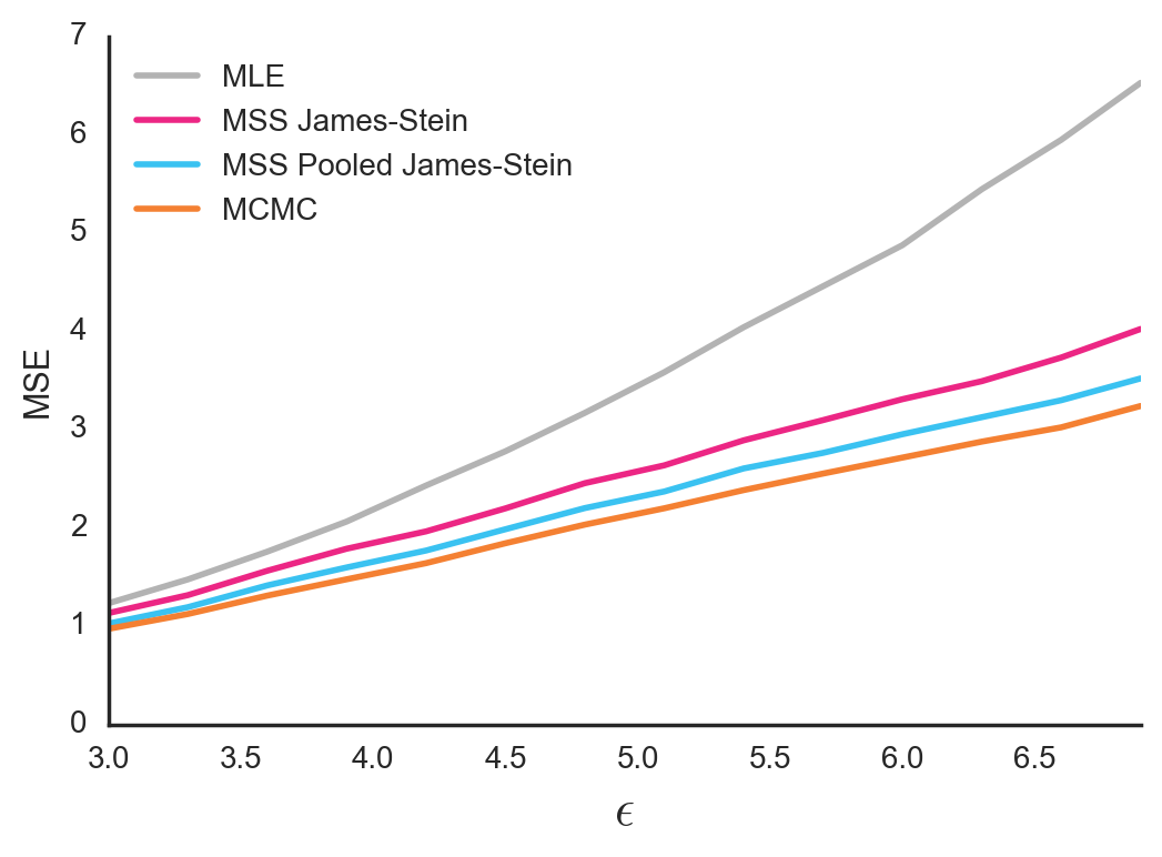
Figure 6. Mean Squared Error between true group means and estimated group means. In this simulation, the \(\epsilon\) parameter for within-group variance of observations is shared by all groups
For simulated data with shared \(\epsilon^2\), MCMC did well, outperforming both the MSS James-Stein estimator and the MSS Pooled James-Stein estimator.
If you don’t care about speed and are willing to write the Stan code, then this is probably your best option. It’s also good to learn about MCMC methods, since they can be applied to more complicated models with multiple variables. But if you just want a quick estimate of group means, then one of the analytic solutions above makes more sense.
Other solutions
There are several other solutions that I did not include in my simulations.
-
Regularization. Pick the set of \(\hat{\theta_i}\)’s that minimize \(\sum{(\hat{\theta_i} - x_i)^2} + \lambda \sum{(\hat{\theta_i} - \overline{X})^2}\). Use cross-validation to choose the best \(\lambda\). This will probably work pretty well, although it takes a bit more work and time than the analytic solutions described above.
-
Mixed Models. Over in Mixed Models World, there’s a whole ’nother literature on how to shrink estimates depending on sample size. They are especially suited for the movie ratings situation because in addition to shrinking the means, they also can correct for rater bias. I don’t really understand all the math behind Mixed Models, but I was able to use lme4 to estimate group means in simulated data under the assumption that the group means are a random effect. This gave me slightly different results compared to the James-Stein / Empirical Bayes approach. I would love if some expert who understood this could write an accessible and authoritative blog post on the differences between Mixed Models and Empirical Bayes. The closest I could find was this comment by David Harville.
-
Efron and Morris’ generalization of James-Stein to unequal sample sizes (Section 3 of their paper). I thought this paper was difficult to read. A more accessible presentation can be found at the end of this column. The Efron and Morris approach is a numerical solution that seemed to work reasonably well when I played around with it, but I didn’t take it very far. If you want to implement it, be sure to prevent any variance estimates from falling below zero. If one of them does, just set it to zero and then compute your estimates of the means. That being said, I feel like if you’re going to go with a numerical solution, you may as well just go with MCMC.
-
Double Shrinkage. When we think that different groups not only have different sample sizes, but also different \(\epsilon_i\)’s, we are faced with an interesting conundrum. As shown above, the MSS James-Stein Estimator outperforms the MSS Pooled James-Stein Estimator, because it computes \(\hat{\epsilon_i}\)’s specific to each group. However, these estimates of group variances are probably noisy! Just like we don’t trust the raw estimates of group sample means, why should we trust the raw estimates of group sample variances? One way to address this is to use Zhao’s Double Shinkage Estimator, which not only shrinks the means, but also shrinks the variances.
-
Kleinman’s weighted moment estimator. Apparently this was motivated by groups of proportions (i.e. the Rotten Tomatoes case), but the estimator can be applied generally.
Conclusion
Which method you choose depends on your situation. If you want a simple and computationally fast estimate, and if you don’t want to assume that the group variances \(\epsilon^{2}_i\) are identical, I would recommend either the MSS James-Stein Estimator or the Double Shrinkage Estimator if you can get it to work. If you want a fast estimate and can assume all groups share the same \(\epsilon^{2}\), I’d recommend the MSS Pooled James-Stein Estimator. If you don’t care about speed or code complexity, I’d recommend MCMC, Mixed Models, or regularization with a cross-validated penalty term.
Acknowledgements
Special thanks to the many people who responded to my original question on Twitter, including: Sean Taylor, John Myles White, David Robinson, Joe Blitzstein, Manjari Narayan, Otis Anderson, Alex Peysakhovich, Nathaniel Bechhofer, James Neufeld, Andrew Mercer, Patrick Perry, Ronald Richman, Timothy Sweetster, Tal Yarkoni and Alex Coventry. Special thanks also to Marika Inhoff and Leo Pekelis for many discussions.
All code used in this blog post is available on GitHub.