Independent t-tests and the 83% confidence interval: A useful trick for eyeballing your data.

01 Dec 2014

Like most people who have analyzed data using frequentist statistics, I have often found myself staring at error bars and trying to guess whether my results are significant. When comparing two independent sample means, this practice is confusing and difficult. The conventions that we use for testing differences between sample means are not aligned with the conventions we use for plotting error bars. As a result, it’s fair to say that there’s a lot of confusion about this issue.

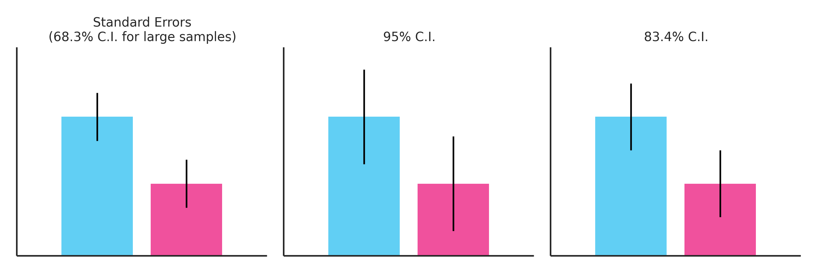
Some people believe that two independent samples have significantly different means if and only if their standard error bars (68% confidence intervals for large samples) don’t overlap. This belief is incorrect. Two samples can have nonoverlapping standard error bars and still fail to reach statistical significance at \(\alpha=.05\). Other people believe that two means are significantly different if and only if their 95% confidence intervals overlap. This belief is also incorrect. For one sample t-tests, it is true that significance is reached when the 95% confidence interval crosses the test parameter \(\mu_0\). But for two-sample t-tests, which are more common in research, statistical significance can occur with overlapping 95% confidence intervals.

If neither the 68% confidence interval nor the 95% confidence interval tells us anything about statistical significance, what does? In most situations, the answer is the 83.4% confidence interval. This can be seen in the figure below, which shows two samples with a barely significant difference in means (p=.05). Only the 83.4% confidence intervals shown in the third panel are barely overlapping, reflecting the barely significant results.

To understand why, let’s start by defining the t-statistic for two independent samples:

\[\begin{align} t = \frac{\overline{X_1} - \overline{X_2}}{\sqrt{se_1^2 + se_2^2}} \end{align}\]

where \(\overline{X_1}\) and \(\overline{X_2}\) are the means of the two samples, and \(se_1\) and \(se_2\) are their standard errors. By rearranging, we can see that significant results will be barely obtained (\(p=.05\)) if the following condition holds:

\[\begin{align} \overline{X_1} - \overline{X_2} = 1.96\times\sqrt{se_1^2 + se_2^2} \end{align}\]

where 1.96 is the large sample \(t\) cutoff for significance. Assuming equal standard errors (more on this later), the equation simplifies to:

\[\begin{align} \overline{X_1} - \overline{X_2} = 1.96\times{\sqrt{2}}\times{se} \end{align}\]

On a graph, the quantity \(\overline{X_1} - \overline{X_2}\) is the distance between the means. If we want our error bars to just barely touch each other, we should set the length of the half-error bar to be exactly half of this, or:

\[\begin{align} 1.386\times{se} \end{align}\]

This corresponds to an 83.4% confidence interval on the normal distribution. While this result assumes a large sample size, it remains quite useful for sample sizes as low as 20. The 83.4% confidence interval can also become slightly less useful when the samples have strongly different standard errors, which can stem from very unequal sample sizes or variances. If you really want a solution that generalizes to this situation, you can set your half-error bar on your first sample to:

\[\begin{align} \frac{1.96\times{\sqrt{se_1^2 + se_2^2}}\times{se_1}}{se_1^2 + se_2^2} \end{align}\]

and make the appropriate substitutions to compute the half-error bar in your second sample. However, this solution has the undesirable property that the error bar for one sample depends on the standard error of the other sample. For most purposes, it’s probably better to just plot the 83% confidence interval. If you are eyeballing data for a project that requires frequentist statistics, it is arguably more useful than plotting the standard error or the 95% confidence interval.

Update: Jeff Rouder helpfully points me to Tryon and Lewis (2008), which presents an error bar that generalizes both to unequal standard errors and small samples. Like the last equation presented above, it has the undesirable property that the size of the error bar around a particular sample depends on both samples. But on the plus side, it’s guaranteed to tell you about significance.