Why are contrast response functions linear in fMRI and nonmonotonic in EEG?

Contrast response functions (CRFs) describe how a neuron’s firing rate depends on the contrast, or intensity, of a visual stimulus. CRFs are really important for testing theories about how the visual system works, and I’ve spent a lot of time over the past few years trying to indirectly measure them in humans, using EEG and fMRI. The problem, however, is that EEG and fMRI give me very different CRFs.

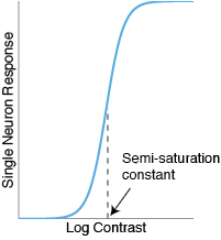
Typically, individual neurons show sigmoidal CRFs. They don’t fire at all for very low contrasts, but they rapidly increase their firing rate at a middle range of contrast. The midpoint of this range is sometimes called the ‘semisaturation constant’. After that, the firing rate tends to level off, or ‘saturate’.

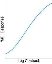
With fMRI, however, I tend to find that the CRFs are mostly linear, not sigmoidal.

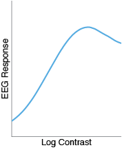
And with EEG, I often find that the CRFs are actually nonmonotonic!

This is weird, and I’m not the first person to notice it. Linear CRFs in fMRI are quite common (e.g. here and here), as are nonmonotic CRFs in EEG (e.g. here, here, here,  and here ). While not all papers show these effects, they certainly seem like real trends. How it is possible that an underlying sigmoidal function in neurons could give rise to such completely different functions measured by fMRI and EEG?

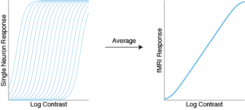
To explain the linear fMRI responses, one idea is that fMRI takes an average over many different neurons, each with a different semisaturation constant. Some neurons saturate early, some saturate late, and when you average them all together you just get a line.

That seems to make sense. But what about the nonmonotonic CRFs in EEG? One idea is that EEG CRFs might reflect the true contrast response functions of individual neurons, many of which are themselves nonmonotonic. While I don’t doubt that this could be a contributing factor, I have trouble believing that this explains all, or even most, of the nonmonotonicity in EEG. Only a small minority of visual cells exhibit this property, and I have seen some _massive _nonmonotonicity in some of my most reliable EEG subjects.

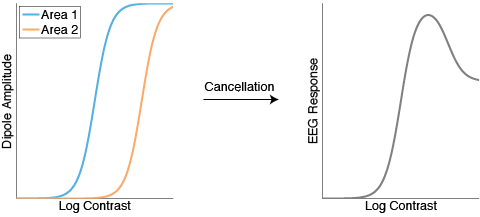
A different hypothesis is that nonmonotonicity is caused by the cancellation of dipoles across cortical sulci or gyri. EEG dipoles are oriented normal to the cortical surface and, since the cortex has so many folds, many of the electrical signals simply cancel each other out.

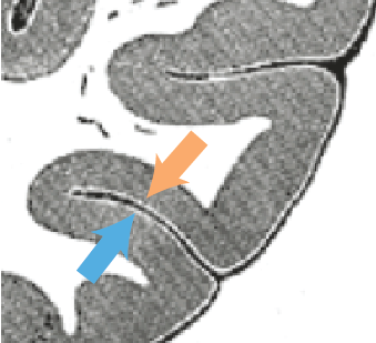
Here’s where it gets interesting. Different cortical areas (e.g. V1 and V2) have different average semisaturation constants. (They tend to get lower the higher you move up in the visual hierarchy). Imagine that two cortical areas with different semisaturation constants live on opposite sides of a sulcus. At medium contrasts, one area will be active and the other will be mostly silent. But at higher contrasts, both areas will have kicked in, and so the overall signal (due to cancellation) will be actually _lower _that at medium contrast. This isn’t my idea, but it makes a lot of sense and I think it deserves more attention.

But wait, the fMRI explanation makes sense, and the EEG explanation makes sense, but how can they both be true? After all, the EEG cancellation story only works if each area’s average CRF is nonlinear: If the average responses were linear (as demonstrated by the fMRI explanation), cancellation of opposite CRFs would just result in more straight lines, right?

Well, yes and no. Using simulations I have found it quite easy to capture both effects. In the fMRI simulation, a perfectly linear CRF emerges only if I assume that the underlying neural semisaturation constants are uniformly distributed, which is quite an unlikely assumption. With any other reasonable distribution (e.g. normal distribution) I get fMRI CRFs that are mostly linear but with a touch of sigmoid. And critically, that touch of sigmoid will drive the dipole cancellation in a way that results in nonmonotonic EEG CRFs.

Below is some Matlab code showing how this works, just a proof of concept. It makes some very, very simplifying assumptions, and I’m sure that the truth is far more complicated.

function [] = crfmodel()

n = 1000; %number of neurons
c = 0:1:100; %contrast levels
c50_std = 30; %stddev of semisaturation constants
c50_mean = [50 70]; %for two visual areas;
c50 = nan(1,n);
for i = 1:2 %loop through two banks of sulcus (two visual areas)
  idcs{i} = (1:n/2) + (i-1)*n/2;
  c50(idcs{i}) = c50_std*randn(1,n/2)+c50_mean(i);
end
[C C50] = meshgrid(c, c50);
R = makeLogistic(C,C50); %Each row is a CRF for a particular neuron
figure

%Single neurons
subplot(1,3,1)
for i = 1:2 %loop through 2 areas
   plot(c,makeLogistic(c,c50_mean(i)));
   hold on
end
ylabel('Single Neuron Response')

%fMRI
subplot(1,3,2);
for i = 1:2 %loop through 2 areas
  CRF_fMRI{i} = mean(R(idcs{i},:),1); %average all neurons in each area
  plot(c,CRF_fMRI{i})
  hold on
end
ylabel('fMRI Response')

%EEG
%Cancellation. Scale factor isn't necessary but reflects that fact that
%some areas are likely to activate more than others.
R_EEG = abs(R(idcs{1},:)-.7*R(idcs{2},:));
CRF_EEG = mean(R_EEG,1);
subplot(1,3,3)
plot(c,CRF_EEG)
ylabel('EEG Response')

function [r] = makeLogistic(c,c50)
r = (1-1./(1+exp(.2*(c-c50))));

And here are the results.

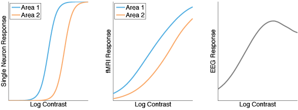
It would be nice if we could go in the opposite direction and reconstruct underlying neural responses from the fMRI and EEG measurements. This seems like a pretty tricky inverse problem, but it might be possible with accurate assumptions about current propagation and the distribution of semisaturation constants.